Locality-sensitive hash functions are becoming increasingly common components of machine learning systems.1 However, Tensorflow does not have good hash function implementations. To address this, I’ve released my own implementations on GitHub. This post describes some of the design considerations.
What hash functions do we need?
We need a hash function for each the four major metric (and near-metric) spaces that are used in machine learning.
- Euclidean space
- Inner product spaces
- Sequences of tokens or strings
- Vectors in other Lp-norm spaces
There are several options for each space, but we will stick to the simplest hash functions. For Lp-norm spaces, we will use the p-stable LSH algorithm. For sequences of tokens and strings, we will use minhash. For inner product spaces, we will use signed random projections.
For the sake of completeness, I’ve included a list of a bunch of alternatives at the end of the post.
Implementing minhash in Tensorflow
Most LSH algorithms only require a few dozen hash functions, but some methods (e.g. the RACE sketch) can require hundreds or even thousands of hashes. To compute a minhash value, we need to use a different hash function for each minhash. This means that we might need a lot of universal hash functions. Tensorflow provides a universal hash function for strings named tf.strings.to_hash_bucket_fast [documentation], which uses Farmhash (a good general-purpose hash function).2 However, it doesn’t allow you to set the internal seed used by the universal hash, meaning that Tensorflow really only has one hash function.
To get around this, we can salt the strings by adding a random suffix to each string before passing it into Tensorflow’s hash function. This causes our single hash function to act like many independent hash functions - one for each salt value. Using this method, it is actually fairly easy to implement minhash in Tensorflow. It can be done in just a few lines of code.
import tensorflow as tf
import random
import string

@tf.function
def minhash(x, num_hashes, num_buckets = 2**32-1, salt_len = 4, seed = 0):
    # Cache and restore RNG state to avoid side-effects for other RNG users.
    state = random.getstate()
    random.seed(seed)
    salts = [''.join(random.choice(string.printable) for _ in range(salt_len))
             for _ in range(num_hashes)]
    salted_strings = [x + s for s in salts]
    hashed_strings = [tf.strings.to_hash_bucket_fast(s, num_buckets)
                      for s in salted_strings]
    min_hashes = [tf.math.reduce_min(h, axis=-1) for h in hashed_strings]
    random.setstate(state)
    return tf.stack(min_hashes)
Because we re-seed the random number generator before generating the salt values, we can be sure that two calls to the function will return the same hash values if the calls use the same seed.
Also, we do not re-generate the salt values very often because of the way that the @tf.function decorator works. This implementation only re-initializes the salt each time the function is traced (not each time the function is called). The salt values are embedded into a Tensorflow graph as constant string tensors the first time the function is called.
Requirements
This implementation is minimalistic and very easy to use, but there are a few drawbacks.
- We re-trace the graph every time we call the function on input tensors with different lengths. Tracing is expensive, and we would ideally want to use the same graph even for sequences of different lengths. We could try to fix it by specifying the
input_signatureof the@tf.functiondecorator, but this only supports tensor arguments and we have default Python arguments (seed, etc). - We need the function to work with single inputs and batched inputs.
- It only works on string inputs, and some workflows use integer tokens.
In this implementation, we address issue 1 by implementing the hash as a class that inherits from tf.Module. This allows us to expose a hash method that exclusively has tensor arguments. Issue 2 is equally straightforward - we can make the function capable of handling both rank-1 and rank-2 input tensors by clever use of the axis keyword argument in tf.math.reduce_min(h, axis=-1).3 However, issue 3 requires a separate implementation for integer tokens, and that raises a problem.
Implementing universal hash functions in Tensorflow
In order to apply minhash to integer tokens, we could just convert the integers to strings and use the method described earlier. This works, but it feels inefficient - why convert an integer to a string, only to hash the string and get back an integer? There are more efficient ways to hash integers.
The standard solution is to implement a mod-prime universal hash function. Given an input integer \(x\), a large prime number \(P\) and uniformly selected integers \(a \in \{1, ... P-1\}\) and \(b \in \{0, ... P-1\}\), the standard mod-prime hash is:
\[H(x) = (ax + b) \mathrm{mod}\quad P\]This method is simple and has nice theoretical guarantees, but it requires a modulo operation (which is expensive on many platforms, including GPU). Many heuristic hash constructions, such as Farmhash or Murmurhash, are faster and have better empirical performance.
Another way to get an integer hash function is by stealing the mixer stage of one of these hash functions. Without going too far into detail, the bit mixer stage (or finalizer) takes an integer and shuffles the bits to obtain an output value. The goal of the finalizer is to evenly spread the output values across the space of integers.
Benchmark
I ran a quick benchmark with Google Colab to see which method is fastest. The benchmark notebook is available on GitHub. You can also run the notebook on Google Colab, if you wish.
For the hashing task, I computed 100 hashes for every entry in a batch of 512 1000-dimensional integer tensors. I repeated this process 500 times on CPU and on a Tesla K80 GPU. The table reports the average hash rates, in megahashes (MH).4
| Method | Hash Rate (CPU) | Hash Rate (GPU) |
|---|---|---|
| 32-Bit Mixer | 57.6 | 90.2 |
| 64-Bit Mixer | 40.2 | 550.6 |
| 32-Bit Mod-Prime | 139.0 | 143.0 |
| 64-Bit Mod-Prime | 62.2 | 63.0 |
The results are surprising on several levels. I would have expected the 32-bit hash functions to be faster than the 64-bit version, especially on GPU. I also expected the mod-prime hash to be slower than the mixer, since bitwise operations are typically faster than affine integer transformations and modular arithmetic.
Neither of my predictions were true: the 64-bit mixer hash was extremely fast (but only on GPU) and the mod-prime hash outperformed the mixer hash in several settings. While many factors could be responsible for the performance gap, I suspect that Tensorflow is aggressively optimized for tensor operations (a common use case) but not for bitwise XOR operations (a relatively rare use case).
Implementing p-stable hash functions in Tensorflow
To compute a p-stable locality-sensitive hash function, we transform an input \(\mathbf{x}\in \mathbb{R}^d\) in the following way.
\[h(\mathbf{x}) = \Big\lfloor \frac{\mathbf{w}^{\top}\mathbf{x} + b}{r}\Big\rfloor\]Here, \(\mathbf{w}\in \mathbb{R}^d\) is a random vector drawn from a p-stable distribution, \(\mathbf{b}\in \mathbb{R}^d\) is a vector drawn from the uniform distribution, and \(r\) is a scalar scaling parameter specified by the user.
Efficient hash projections
The obvious improvement is to compute several hash functions at one time by projecting a batch of N inputs \(\mathbf{X}\in \mathbb{R}^{N \times d}\) through a batch of M hash projections \(\mathbf{W} \in \mathbb{R}^{d \times M}\). This can be done via tf.matmul or tf.tensordot.
import tensorflow as tf

batch_size = 512
dimensions = 128
num_hashes = 100
r = 1.0

# Random input data.
X = tf.random.normal([batch_size, dimensions])
# For Euclidean LSH, use Gaussian vectors (2-stable).
W = tf.random.normal([dimensions, num_hashes])
b = tf.random.uniform([num_hashes], minval=0, maxval=r)
# Compute the hash values.
projs = tf.matmul(X, W) + b
hashes = tf.cast(tf.floor(projs / r), tf.int64)
Batched hash computations are amenable to GPU acceleration because they can be implemented using standard matrix multiplication. For efficiency reasons, we want to do large batches of hash calculations at one time. Therefore, the interface of the hash function needs to accept batched inputs and to output multiple hash codes.
Note about vector inputs: There are situations where we’d like to hash a rank-1 (vector) input. We can accomodate both types of input using tf.tensordot instead of tf.matmul, at a small cost to code readability.
Generating p-stable vectors
The main difficulty with implementing a p-stable hash function is that p-stable vectors are not easy to generate, due to the lack of standard routines to sample from p-stable distributions. Tensorflow is pretty limited when it comes to random number generation - it only provides the ability to generate Gaussian and uniform distributed vectors.
Fortunately, this is all we need. We can transform uniform random vectors into p-stable vectors using a routine by Graham Cormode. The mathematical expressions are fairly complicated, but the implementation is not too difficult.
import tensorflow as tf
import math

# Generate output drawn from a p-stable distribution.
p = 1.0
size = 1000  # Size of output vector.
x0 = tf.random.uniform([size], minval=0, maxval=1)
x1 = tf.random.uniform([size], minval=0, maxval=1)

theta = math.pi * (x0 - 0.5)
w = -1.0 * tf.math.log(x1)
left_denom = tf.pow(tf.cos(theta), 1.0 / p)
left = tf.sin(p * theta) / left_denom
right_base = tf.cos(theta * (1.0 - p)) / w
right = tf.pow(right_base, (1.0 - p) / p)
output = left * right
NaN complications: If we’re unlucky, this implementation can overflow a 32-bit floating point value, resulting in inf or nan hash values. This is more likely to occur for values of p that are close to zero, due to the large exponents. We can fix this problem in two ways:
- Threshold the output and replace
-inf, inf, nanwith large values (e.g. 10e16). Since we will use the vectors for inner product projections, the output thresholds should be a few orders of magnitude smaller than the maximum floating point magnitude. - Limit the range of the uniform distribution to guarantee that overflow cannot occur for a range of p values.5 In practice, we’re unlikely to need values of p smaller than 0.5 for LSH.
Implementing SRP hash in Tensorflow
Signed random projection (SRP) hashes are very similar to p-stable hash functions. We simply generate a Gaussian-distributed vector \(\mathbf{w} \in \mathbb{R}^{d}\) and take the sign for the inner product (or projection) of the input.
\[h(\mathbf{x}) = \mathrm{sign}(\mathbf{w}^{\top}\mathbf{x})\]It is common to clip negative signs to zero to obtain a bit vector instead of a vector of +1 and -1 values.
Should we output a bit vector?
SRP hash functions normally output a bit vector - a sequence of 1s and 0s. For most applications (such as indexing or hash tables), we need a single integer number rather than the array. In a low-level language such as C, it’s easy to shift and pack the bits into an appropriately sized integer. But in a pure Tensorflow implementation in a high-level language like Python, this is a little more difficult. There are two ways to do it:
- Take the inner product of the binary array with an array containing the powers of two.
- Use binary operations to shift and xor bits into the correct position on the output hash code.
Benchmark
Obviously, the solution is to benchmark the two approaches and pick the fastest method. We implemented both methods and tested with a variety of batch sizes and bit lengths. The plot compares the time needed to compute 512 hashes for a batch of 1024 vectors in 128-dimensional space.
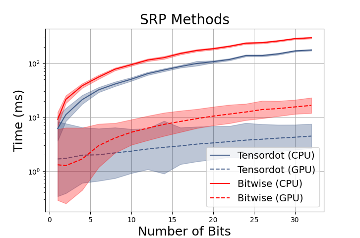
While the binary approach would be more efficient on most platforms, modern deep learning frameworks are designed to take advantage of fast matrix manipulation. If we were compiling the hash implementation to instructions rather than Tensorflow graph operations, the bit shift method would most likely win as it is technically cheaper than floating point multiplication. But in a deep learning framework, it makes more sense to use the fast inner product with GPU acceleration.
Putting it all together
I’ve put together all of these ideas to get the implementation on GitHub. The module is released under the Apache-2 license and is free for research and commercial use.
Testing the functions
We include a test suite for all our hash functions. While testing randomized algorithms can be difficult, it is usually okay to compute a large number of hash values (1000+) for two inputs and empirically verify the LSH collision probability. If the numbers of hash matches are approximately the same as those predicted by the theory (within 2-5%), then the implementation is probably correct. For more guidance on testing randomized algorithms, see this blog post.
List of locality sensitive hash functions
Here is a non-exhaustive list of alternative hash functions for common metric spaces. Note that most methods can be used for more than one metric. For example, there’s a lot of overlap between hash functions for high-dimensional inner product spaces and token/string representations. The reason is that we can approximate the inner product in high dimensions by binarizing the vector, then computing the Jaccard index. These approximations go the other direction too: we can usually embed the Hamming space into the Euclidean space.
For this reason, methods like bit sampling, minhash, permutation hashing and DOPH can be applied to both strings and high-dimensional vectors.
L1, L2 and other Lp-norm spaces
P-stable projection hashing: Partition the data by thresholding the inner product of the input with a random vector drawn from a p-stable distribution. This amounts to taking an inner product and then rounding the result.
Data-dependent hashing: Select partitions that cover dense subsets of the data (Euclidean and Hamming spaces). For Euclidean and Hamming spaces, this is done by partitioning the space into near-hemispheres (called sperical caps), preferring caps that contain large fractions of the dataset. The resulting hash function is sometimes called the Spherical LSH.
Inner product spaces
Signed random projections (SRP): Partition the data according to the sign of the inner product between the input and a random Gaussian vector. This process produces a binary output. Repeat this process multiple times to obtain a multi-bit hash value.
Sparse random projections Similar to SRP, but we randomly zero out some of the components in the projection vector. We can also use binary projections, where the vectors are drawn from +/-1, instead of the normal distribution. A variety of sparsity ratios will work, but a common strategy is to simply delete two thirds of the entries. However, we can use even more aggressive sparsity ratios in most cases.
Super-bit LSH: Similar to SRP, but select orthogonal Gaussian projection vectors rather than independent Gaussian vectors. That is, we construct several projections at a time by choosing components from a randomly-oriented orthonormal basis.
Cross-Polytope LSH: This method applies many Gaussian random projections to the input, then finds the hash value via a near-neighbor lookup on basis vectors. This differs from previous constructions in the sense that many projections are used for each hash function - one for each dimension of the input. The resulting hash function is often referred to as the cross-polytope LSH, since the partitions are found by finding the nearest corner of a randomly-oriented L1 norm ball (a polytope).
Asymmetric LSH: Hash the data and the query using different hash functions. This yields a hash function that collides points with large inner products but introduces additional variance to the hashing process.
Bit sampling: Given a binary vector, randomly sample a dimension and output the corresponding bit from the vector. This hash is sensitive to inner products over binary data (i.e. the Hamming distance).
Tokens and strings
Minhash is a method to group together strings and sets of tokens based on their Jaccard similarity (a type of overlap score). Because minhash is a very influential idea in search and (more recently) in genomics, most of the LSH functions for strings and tokens are minhash derivatives.
Minhash: The idea behind minhash is to compare two sets of tokens by selecting a random token and checking to see whether both sets contain the token. Conceptually, minhash does this by constructing a randomly-ordered “preference list” from the entire space of possible tokens. Given an input set of tokens, minhash computes the hash value by outputting the ID of the token with the highest preference. Of course, the actual process is more efficient, but it’s too complex to describe here.
One permutation hashing: For minhash, we had to compute a randomly-ordered preference list (or permutation) among the items. If we want to compute multiple minhash values, we have to compute multiple permutations. Despite cheap tricks to get the permutation, it’s still expensive if we have to do it hundreds of times. The “one permutation hashing” method provides a way to get multiple minhash values from the same permutation. This is done by cutting the preference list into chunks - one chunk for each minhash.
Densified one permutation hashing (DOPH): The one permutation hash works well, but only for large sets that contain many items. Otherwise, some of the chunks in the preference list might be empty, leading to degenerate minhash values. DOPH fixes this problem via a densification trick that extends the method to work on sparse data.
Containment Minhash: Containment minhash is an improvement to minhash that has lower variance when comparing sequences with imbalanced lengths. The key idea behind containment hashing is to only check the tokens that are in the smaller set (i.e. restrict the preference list). This improves our estimate of the overlap between the large and small sets.
Weighted Minhash: Weighted minhash is a technique for situations where some tokens are more important than others. It is sensitive to the weighted Jaccard similarity - the hash value is more likely to be determined by the presence / absence of important tokens than unimportant ones.
Notes
-
High-profile conferences such as NeurIPS and ICML have published several algorithms to train networks with LSH (SLIDE and MONGOOSE), perform negative sampling with LSH, improve transformers (the Reformer architecture), and accelerate tasks in kernel-matrix algebra and density estimation. ↩
-
You can figure this out by reading the implementation of this function on GitHub (which is in C), and following the reference to Fingerprint64 (which uses Farmhash). ↩
-
If you use compatibility mode to support Tensorflow 1.x, then it is harder to accept rank-1 and rank-2 inputs. The best method is to check the rank of the input tensor and use
tf.expand_dimsto add an outer batch dimension. ↩ -
To compare these results with those from the standard smhasher suite, multiply the hash rate by 4 or 8 to get the MB/sec rate. If you do this, note that we are evaluating on very small integer keys. ↩
-
Initialization bounds are better if you are using compatibility mode to support Tensorflow 1.x, since some of the operations can throw errors if called with
nan/inf/-infarguments. This does not appear to be a problem in Tensorflow 2.x. ↩