This is the companion blog post for our paper “Sub-linear RACE Sketches for Approximate Kernel Density Estimation on Streaming Data.” The main contribution of the paper is the Repeated Array of Count Estimators (RACE) sketch, which is an efficient way to represent data distributions in a few megabytes. The goal of the paper is to perform kernel density estimation, which computes a sum over N data points \(\{x_1, x_2, ... x_N\}\):
\[f(q) = \sum_{i = 1}^N k(x_i,q)\]This is called a kernel sum and the function \(k(x,q)\) is called the kernel. If we want to compute the sum directly, we have to evaluate the kernel N times - once for each point in the dataset. This is really inefficient.
We obviously want to reduce the computation, but the memory is actually a serious issue too. Think about what happens if each element in the dataset is a 256-dimensional vector of 32-bit floating point numbers (a common output dimension for neural embedding models). If N is one million, we need one gigabyte of RAM to compute the sum. If N is in the billions, which can totally happen at places like Google and Amazon, we need terabytes of RAM.
Why are kernel sums important?
Kernel sums are the backbone of a time-honored list of machine learning techniques known as kernel methods. Kernel methods used to be the hot topic in machine learning until they were displaced by deep neural networks, but they’re still important and used by many people. In the paper, we focus on kernel density estimation (KDE).
Kernel density estimation is a way to approximate the distribution of a dataset just by looking at the points in the dataset. KDE does not make very many modeling assumptions, so it’s a fairly general technique to model the probability distribution that generated your data. To understand KDE, we need some intuition about the kernel function \(k(x,q)\). This function should be large when \(x\) and \(q\) are similar and small when they are not. If the kernel has these properties, we call it a similarity kernel because it measures whether \(x\) and \(q\) are close to each other.
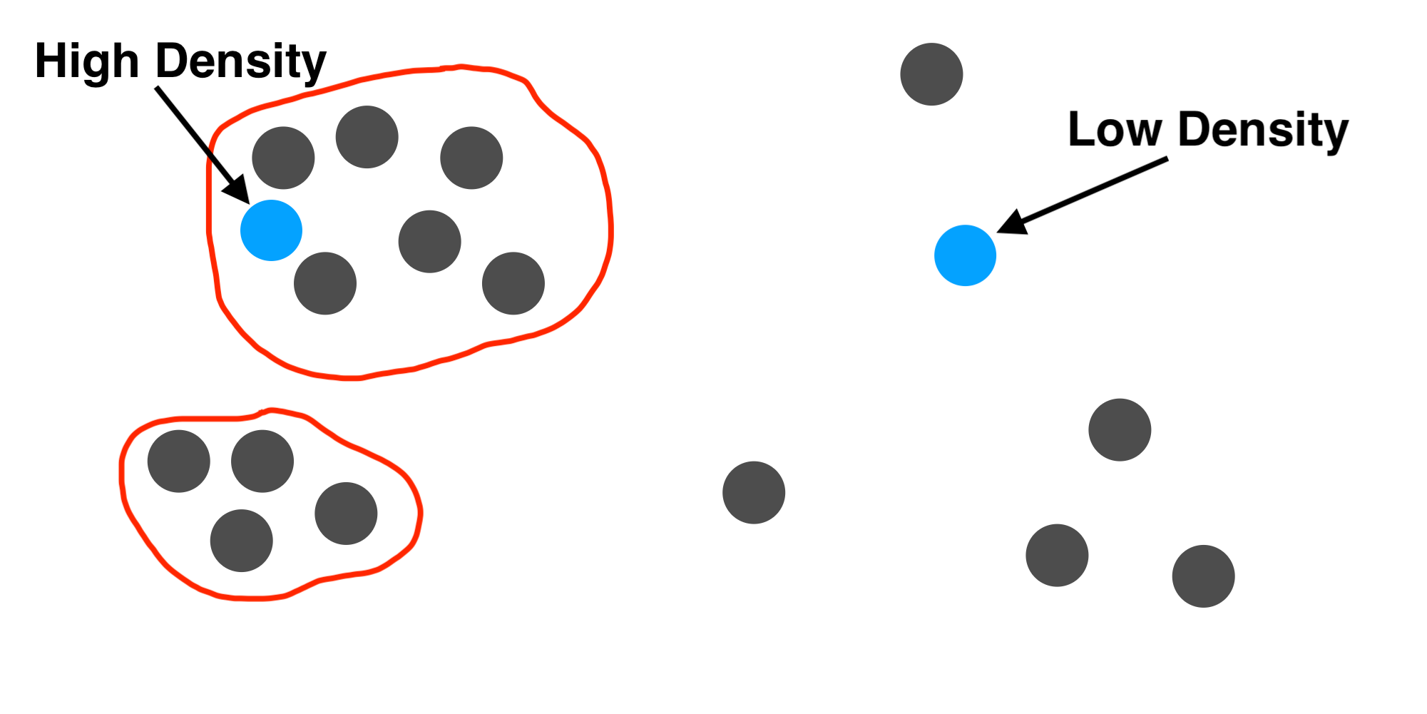
By adding together all of the \(k(x,q)\) values, we can measure whether \(q\) fits in with the observed data. If \(q\) is similar to lots of examples from the dataset, many of the kernel values will be large and we will get a large sum. If \(q\) is not similar to any examples, the kernel sum will be small. The KDE model just divides the sum by a normalization constant so that the density integrates to 1. The model assigns a high probability density to a query if it is close to many examples and a low density otherwise.
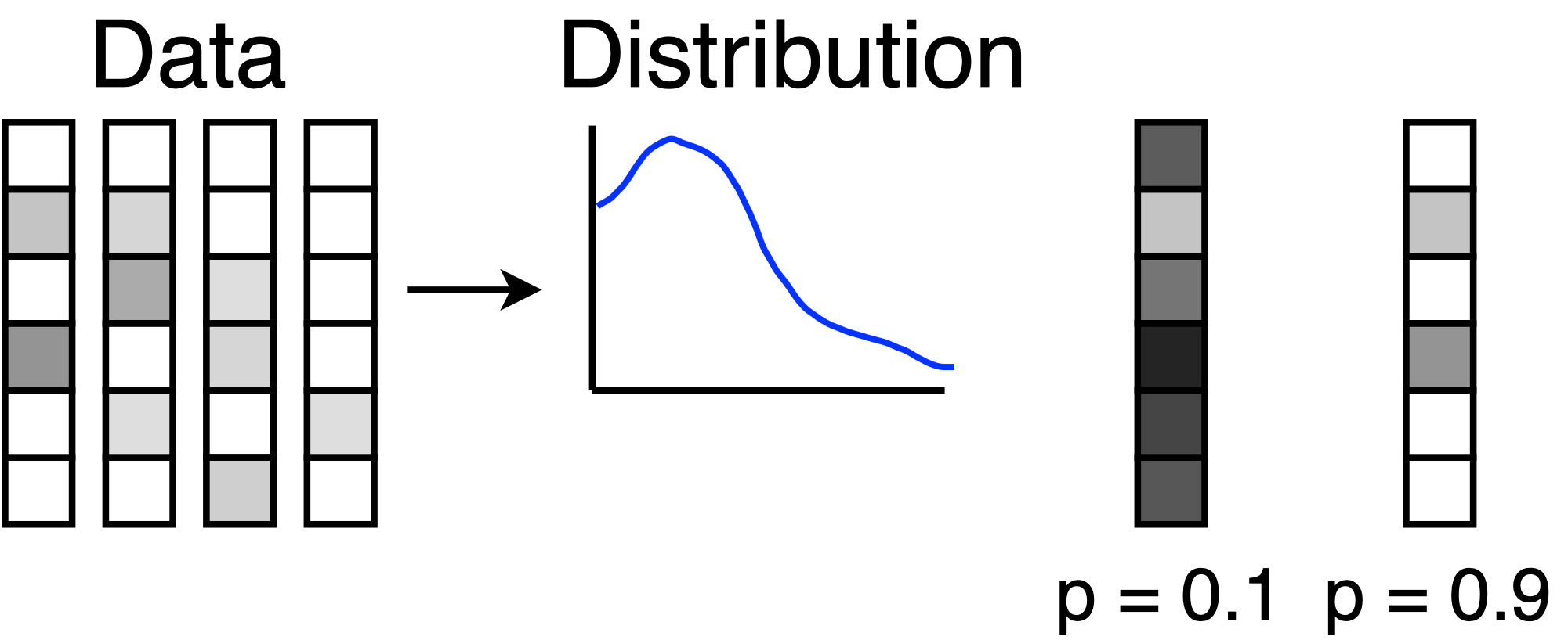
One way to use the KDE model is to detect anomalies. If the model assigns a low probability to a query, then the query does not resemble any examples from the data. In the picture, the anomalous query has a probability of 0.1 because it is different from all the data points. The other query has a probability of 0.9 because it is highly similar to the data.
The RACE Sketch
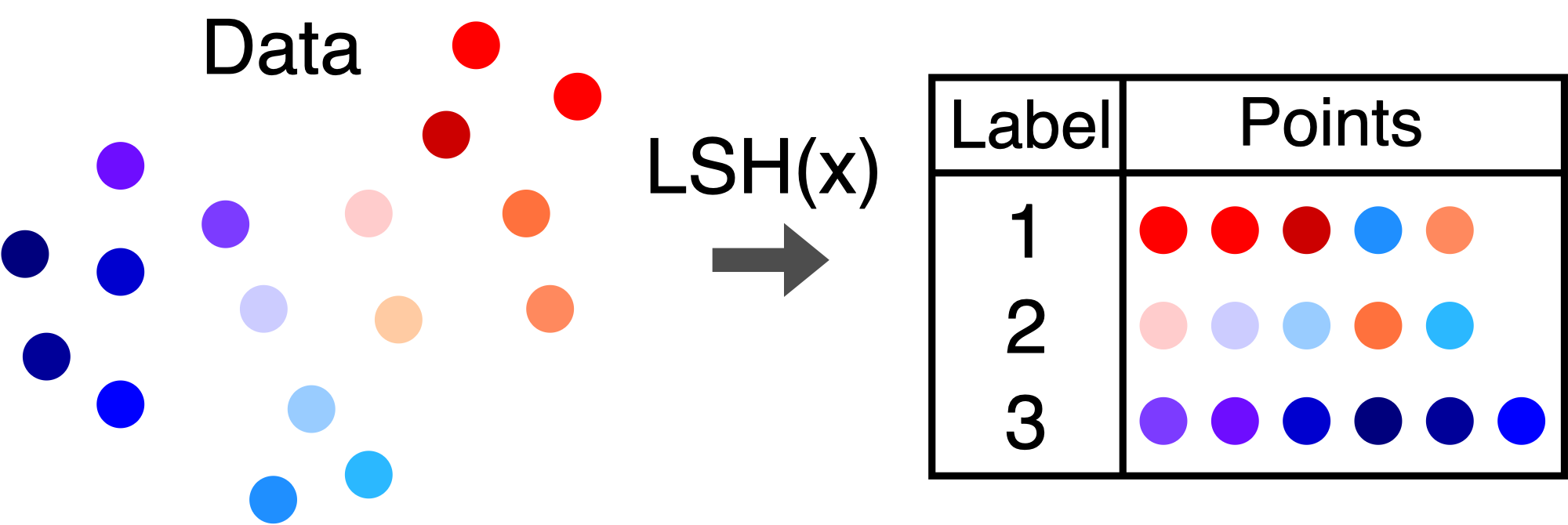
The RACE sketch is a 2D array of integers that is indexed using a locality sensitive hash function. Locality sensitive hashes are functions that label data points with integers. If two points are similar, then there is a high probability that they will have the same label. If the points are far apart, there is only a small probability of having the same label.
If this sounds an awful lot like a kernel, you are right - the collision probability of an LSH function is a valid kernel function. We call these functions LSH Kernels. For example, here are the LSH kernels that correspond to the signed random projection and 2-stable (Euclidean) LSH functions.
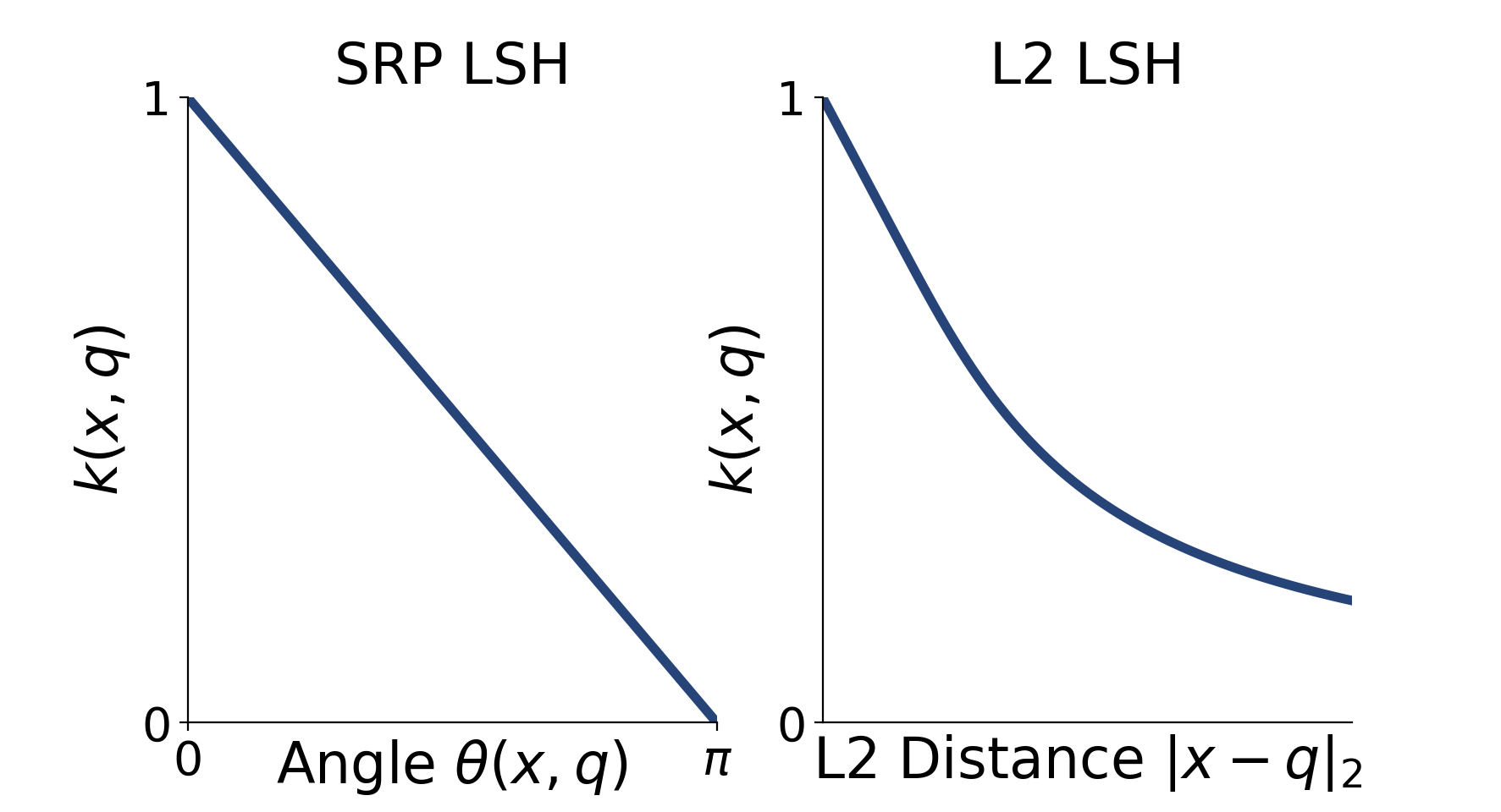
One of the observations in our paper is that you can add together different LSH kernels to get functions that resemble popular kernels that people already use.
Constructing the Sketch
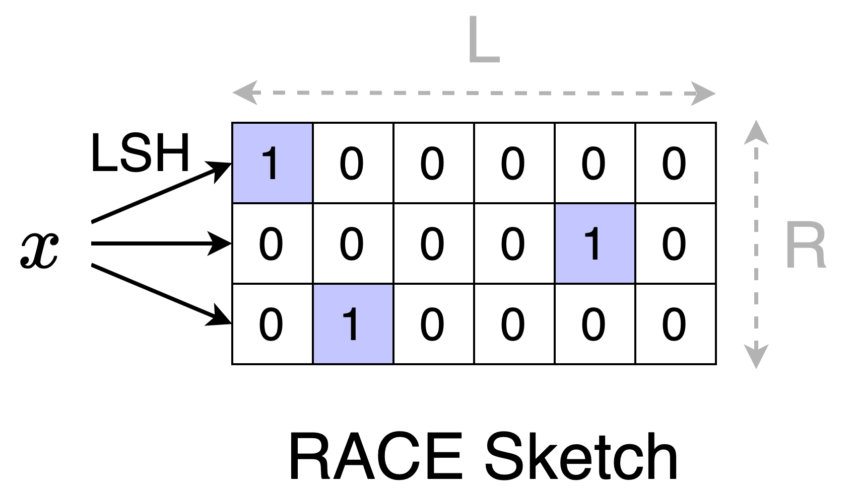
To construct a RACE sketch, we start with an \(R \times L\) array of zeros and \(R\) LSH functions. Each row of the array is indexed using the corresponding LSH function. To add an element \(x\) to the sketch, we hash \(x\) to get \(R\) LSH values and we increment the counters at those indices. The picture shows how to insert \(x\) with LSH values [0, 4, 1] to a (3 x 6) sketch.
Since addition is commutative, we can do the increments in any groupings or order. This means that we can split the dataset into two (or more) chunks, construct a sketch for each chunk, and then merge the chunks by adding the corresponding counters.
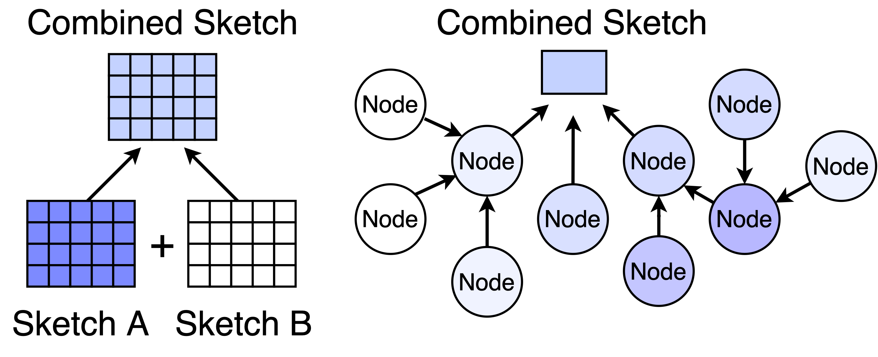
In fact, we can go beyond merging two sketches and distribute the workload over lots of devices in a network. To get the summary of the whole dataset, we aggregate the sketches along the nodes of the network.
Querying the Sketch
Querying the sketch is very similar to adding an element to the sketch. We compute the hash values and access the corresponding locations in the array, but we take the average of the values and do not increment.
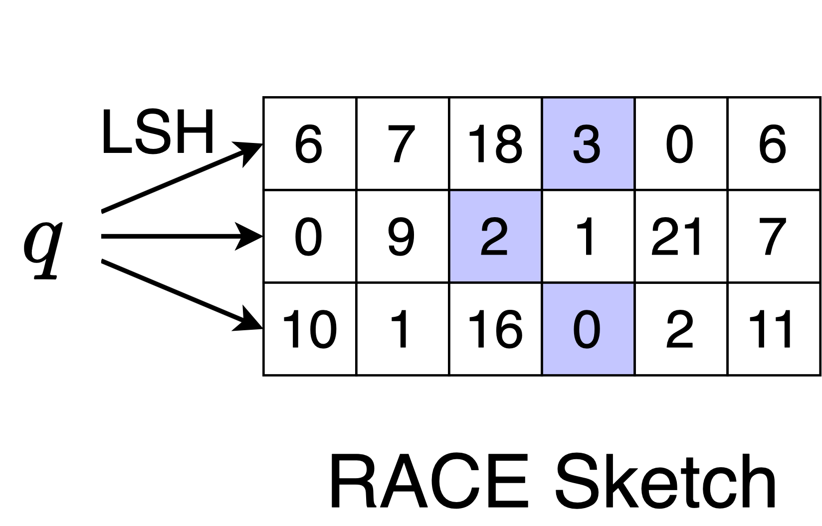
Here, the query lands on [2, 3, 0], so we report that
\[\sum_{i=1}^N k(x,q) \approx 1.6\]Why does this measure density? If a query is similar to many points from the dataset, then it will have the same LSH label as many points. This means that the query will land in a cell that has a large count value. If the query has a low average count value like in the example, then it is far from many points in the dataset. Mathematically, the sketch estimates the sum of LSH collision probabilities. Since the collision probability is a kernel, we can do kernel density estimation with the sketch.
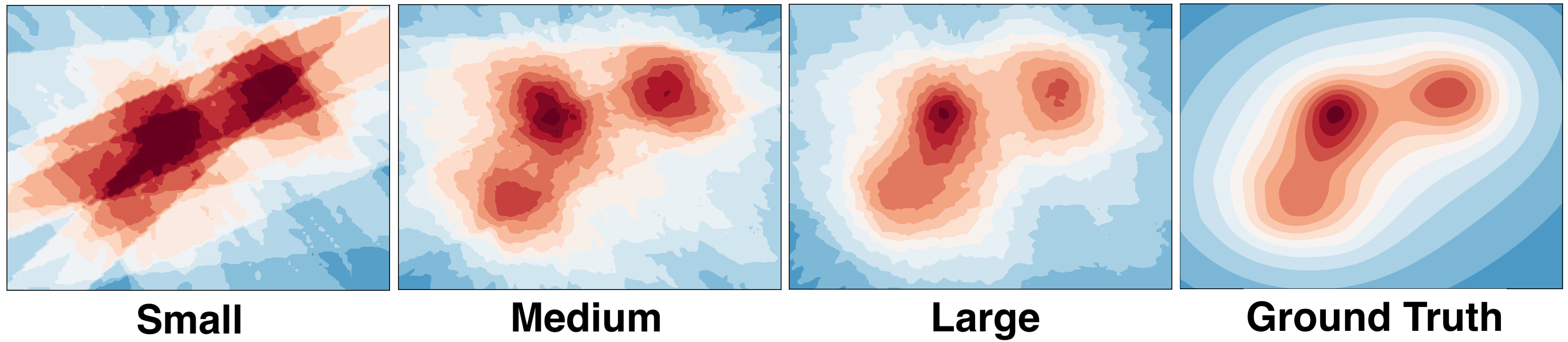
How do I choose L and R? There is a theorem in the paper that relates the size of the array to the error of the approximation. For most applications, it is reasonable to choose R between 100 and 1000 with L up to 5000. As you can see in the picture, increasing the size of the sketch also increases the quality of the approximation. The small, medium and large sketches were constructed using R = 15, 50, and 100. We used L = 40 for all the plots. Here is a useful design formula:
\[|\mathrm{KDE}(q) - \widehat{\mathrm{KDE}}(q)| \approx \frac{1}{\sqrt{R}}\]How can I normalize for KDE? In KDE, you will want to divide by N. To get N, simply take the row sum over the sketch - since each point is added to exactly one cell in each row, we can recover N by adding the counts of all the cells.
How do I adjust the bandwidth of the kernel? You can adjust the KDE bandwidth by changing the LSH function. See the paper for details.
Experiments
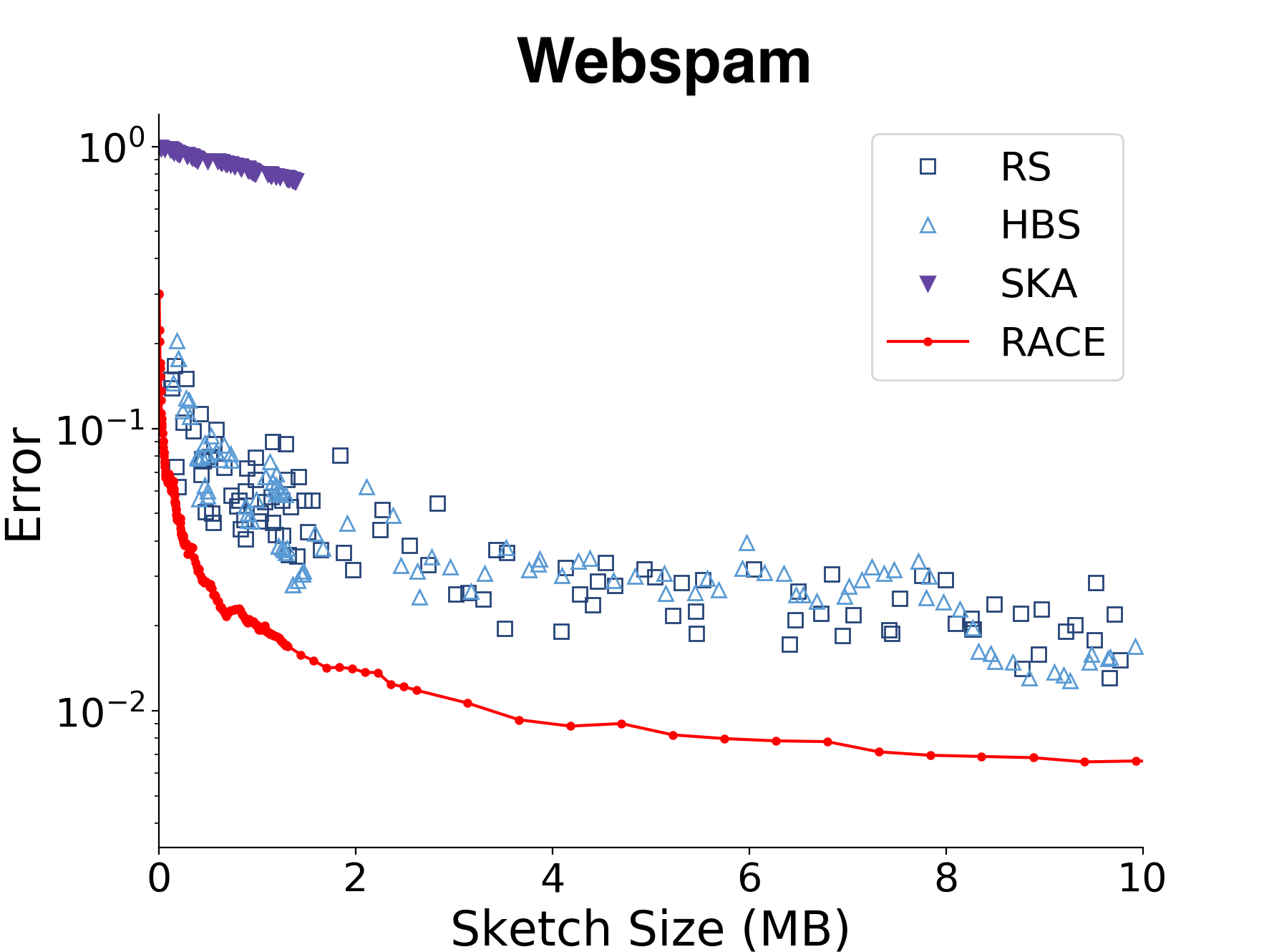
There are lots of experiments in the paper, but here is a comparison of different KDE methods on the webspam dataset with the Euclidean kernel. The webspam dataset has 350k data points and 2.3M dimensions (but a much lower intrinsic dimensionality).
Here is a comparison with the angular (SRP) kernel on hyperspectral imaging data from Pavia, Italy. There were about 750k data points with 100 dimensions in this dataset.
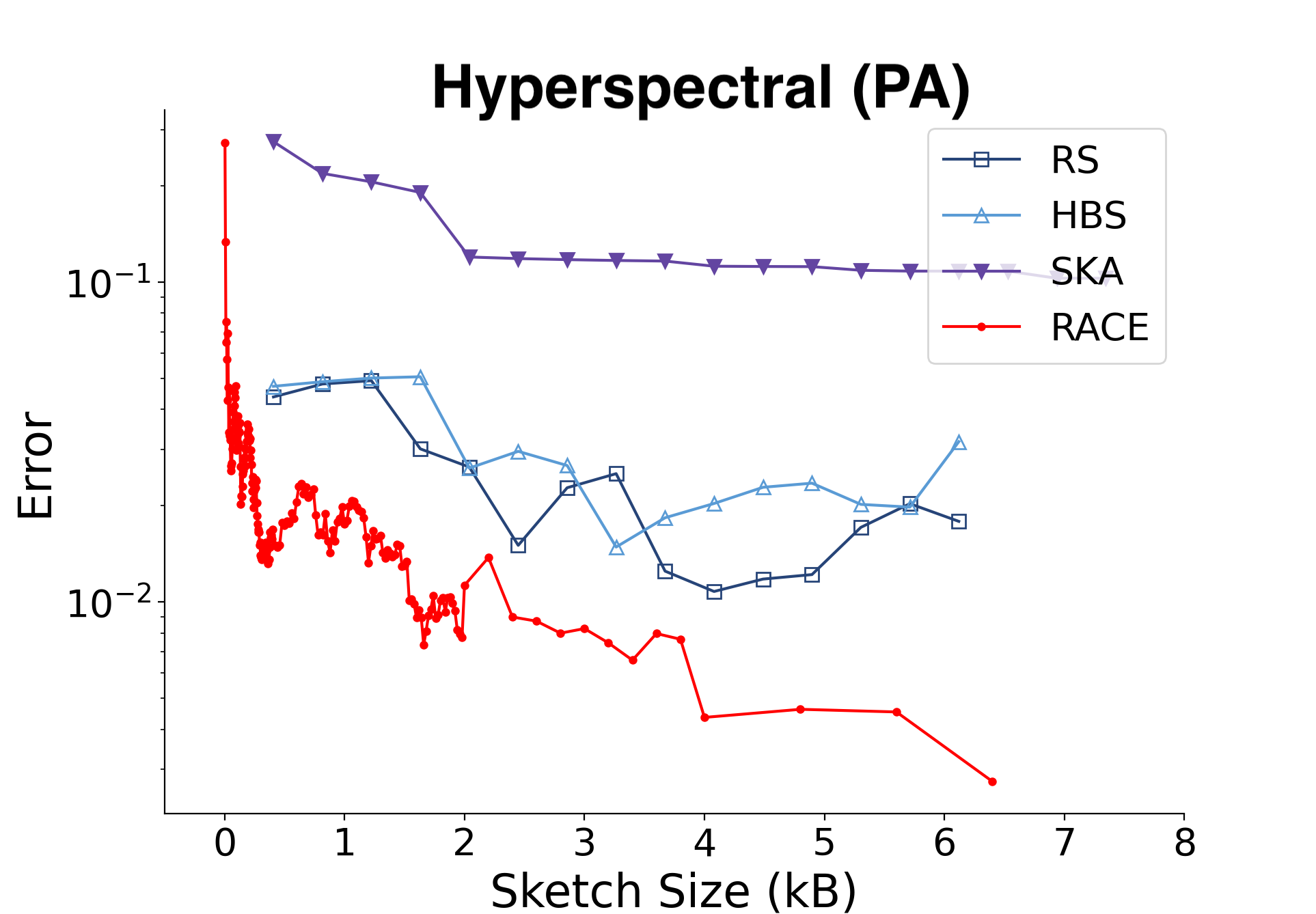
RACE can estimate the kernel sum to within 1% of the true value using about 4 MB of RAM for the Euclidean kernel and a few kilobytes for the angular kernel.
Some LSH Kernels are easier than others
The length L of the sketch is determined by the number of values that the LSH function can output. But some LSH functions can output an infinite number of different integers. It would make sense that these LSH kernels are harder to deal with, since we have to “squeeze” an infinite number of possible outputs into just L different locations in the array.
We address this in the paper when we talk about the rehashed RACE estimator for LSH functions with unbounded support. Since there are an infinite number of possible outputs, we rehash them onto the L locations. The rehashed RACE sketch has different theoretical guarantees than the non-rehashed version. There are three interesting observations:
1. The spread of the dataset determines L
You can think of each cell in the RACE sketch as corresponding to a region in space that contains similar objects. If our dataset covers more space, the sketch has more regions and we need a larger value of L. Therefore, spread out datasets require a larger sketch than tightly packed ones.
2. We pay for kernel bandwidth using L
For all known LSH kernels, decreasing the bandwidth makes the LSH function output a larger number of values. To accommodate the larger number of hash values, we need to increase L. This means that the price of a finer-grained density estimate is an increase in the sketch size.
3. Some metric spaces are easier than others
If the points are in a bounded metric space, then the kernel sum problem is easier. A bounded space is one where there is a maximum distance between points. For example, the angle between two vectors cannot be greater than 180 degrees (when the vectors are pointing in opposite directions), but the distance between points can be arbitrarily large. This is why the angular LSH kernel requires kilobytes when the Euclidean LSH kernel requires megabytes.
Isn’t high-dimensional density estimation hard?
Kernel density estimation has a bad reputation for being difficult and even intractable in high dimensions. You could argue that even though we have a good approximation of the kernel sum, the kernel sum itself is a poor approximation of the density. It’s true that KDE has a slow convergence rate in high dimensions. However, this problem can be cured by a preposterous amount of data. The convergence rate of the L2 function error between the estimate and the real density is:
\[\mathrm{error} = O\left(N^{-\frac{4}{4+d}}\right)\]By stating this result outright, we’re skipping a lot of details. For a full discussion, I suggest “Multivariate Density Estimation” by David Scott - it’s the most comprehensive book that I know of for the density estimation problem. The main takeaway is that high-dimensional density estimation is plagued by the curse of dimensionality. If d is large, we have to use a big dataset (large N) to get a good density estimate. With existing techniques, this would not be worth the computation time or the terabytes of RAM needed to compute the sum and it would indeed be intractable. However, we can construct RACE sketches with a distributed streaming algorithm that only requires a few megabytes of space. We can harness the power of massive distributed computations to do KDE at a large enough scale that the convergence rate is no longer a problem.
Applications
We are still exploring the applications of the RACE sketch, but we can already see that it is useful to have such a simple and fast method for density estimation. So far, we have used RACE to process and downsample large genomic data streams, LLM pre-training corpora, and to implement compressed near neighbor search. RACE can also be used to estimate a class of divergences between dataset distributions, which is useful for federated learning, data selection, and other machine learning applications.