The histogram is a data summary that is widely used across science, engineering, finance and other areas. Histograms are often the first thing you look at when exploring a new dataset or problem. You can use them to visualize the distribution, identify outliers and do all sorts of other useful things.1
But histograms are hard to build if we don’t have access to the full dataset up front. We need some tricks to build histograms over streaming data, where values arrive one at a time. This post will explain the tricks.
Why do we need streaming histograms?
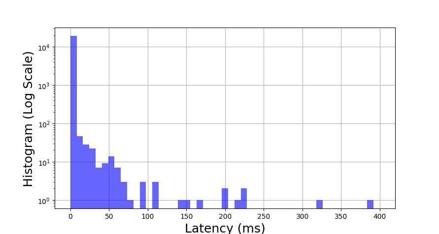
Usually, we compute a histogram over a static set of data. However, sometimes we want to compute a running histogram over a stream of values. For example, we might be running a web service that responds to requests from customers, and we’d like to monitor the health of the service based on how long it takes to serve each customer. In other words, we want to find the latency histogram.
One approach is to just add new values to the histogram as new data points become available. The problem with this approach is that the global histogram might not reflect recent events.
For example, suppose we log all the request latencies throughout the day, but the server crashed for the last ten minutes. The last ten minutes’ worth of service times will be really high (at least ten minutes), but we might miss them because the vast majority of values in the histogram came from before (when the service was healthy). By the time the unserved requests do show up, it might be too late to fix the problem without consequences.
We need a type of histogram that prioritizes recent data and ignores old data.
Windowed Histograms
Windowed histograms are easy to understand but not very nice to implement. The output of a windowed histogram is simply the histogram of the W most recently seen points from the stream, where W is the window size. By deleting old points from the histogram, we allow the histogram to adapt to changes in the distribution of inputs from the stream.
The main problem is that we need to store a buffer of the W most recently seen points from the stream. Unfortunately, there is no way to avoid this O(W) space requirement.2 This can be prohibitive for large windows, since we have to store a huge rotating buffer of input points.
Decayed Histograms
Decayed histograms are a solution to the space problem that we encountered with windowed histograms. The idea is to slowly decrease the influence of a contribution over time, until eventually its contribution is negligible.
The most common way to do this is via exponential decay. Each time we update the histogram, we scale the existing counters by constant multiplier (smaller than 1). This process reduces the contributions of older counters, since they have been scaled by the multiplier many times. But the distinction between a value that’s “in the window” and “outside the window” is much less clear than with windowed histograms.
This raises some questions.
- How long does it take for the contribution of a point to become negligible?
- How do we set the decay rate so that our histogram focuses on the W most recent points?
- If we want a normalized histogram, what value should we normalize by?
Question 1: Half-Life of a Point
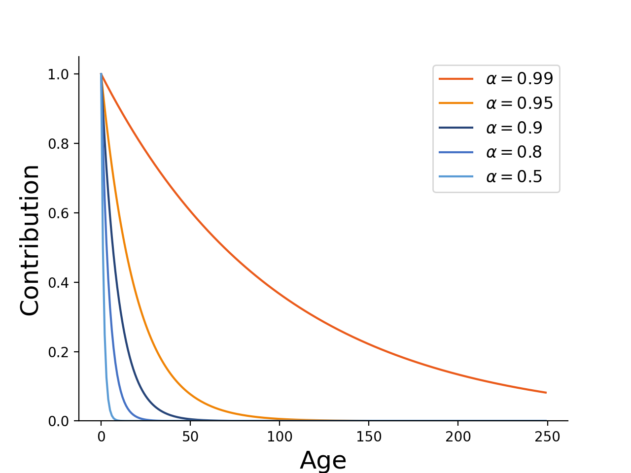
Say we increment a histogram bin by 1. What happens to this increment in future time steps? After one, two or T more inputs, this increment will be worth:
\[\alpha, \alpha^2 ... \alpha^T\]The pattern is pretty clear - the contribution decays by a multiplicative rate every time we add a new value to the histogram.
We can use the change of base formula to transform this into a more familiar exponential form.
\[1 \times e^{T \ln \alpha}\]Now, the contribution of the point is in the traditional half-life formula commonly encountered in physics, biology and chemistry. The decay constant and half life are:
\[\lambda = - \ln \alpha \quad t_{1/2} = \frac{\ln 2}{\lambda}\]As an example, if we multiply by 0.95 then the contribution of an input to the histogram will drop to 0.5 after 13 inputs. If we increase the multiplier to 0.99, then points stick around longer: roughly 69 steps are needed to halve the counter.
Note: Because multiplication distributes over addition, the scaling property distributes over all the increments. Each input decays at the same exponential rate, but the counters in the histogram represent the sum of decayed increments. For this reason, we no longer need O(W) space to represent the streaming histogram - we can just scale the counter sums at every iteration and rely on the distributive property of addition.
Question 2: Setting the Decay Rate
Now that we understand how the contributions decay over time, we would like to know how to set the decay rate. This is useful because it allows us to have the histogram only pay attention to a certain number of recent values. To do this, we will find the window that is responsible for the majority of the contributions to the histogram’s output.
We will start by taking a look at the total value of all contributions (the sum over all the histogram bins). We will say that the exponential histogram has a window size of W if the most recent W inputs are responsible for a large amount of the total (perhaps 95%).
At time T, the total sum of all increments is:
\[\sum_{t = 0}^T \alpha^t\]We recognize this as a geometric series sum. We are interested in long-running streams, so we would like to know the steady-state value of this sum. That is, we want to know the value of the sum as T grows arbitrarily large. This value can be found by taking a limit, resulting in a well-known formula that’s taught in most calculus classes.
\[\lim_{T\to\infty} \sum_{t = 0}^T \alpha^t = \frac{1}{1 - \alpha}\]If we allow the histogram to run on a very long data stream, the sum over all the bins will eventually reach this steady state value due to the convergence of the geometric series sum. Now let us consider the sum, but restrcted to only the most recent W points. This is a partial geometric series sum over the first W terms in the series, and there’s a nice closed-form expression for its value.
\[\sum_{n=0}^W \alpha^n = \frac{1 - \alpha^W}{1 - \alpha}\]We are interested in the number of terms needed for the partial sum to represent most of the full sum - these are the points that contribute most strongly to the output value and are therefore the points that should be considered “inside the window.”
For example, maybe we are using a multiplier of 0.99 and we want the partial sum to be 95% of the full sum. How many terms are necessary to make this happen? We can find out by setting the partial sum equal to 95% of the full sum and solving for W.
\[\frac{1 - 0.99^W}{1 - 0.99} = \frac{0.95}{1 - 0.99}\] \[1 - 0.99^W = 0.95 \Rightarrow 0.99^W = 0.05\] \[W = \frac{\log 0.05}{\log 0.99} = 298\]From this, we see that the 95% window size is 298 when we use \(\alpha = 0.99\). In other words, inputs older than 298 steps are collectively only worth 5% of the total mass in the histogram. Now we’re going to generalize this result for percentages other than 95% and multipliers other than 0.99. If we want to get to a fraction \(1 - \delta\) of the total, we need to have the following number of terms in the sum.
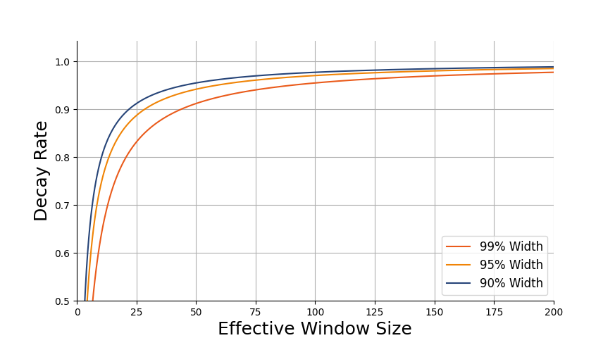
\[\frac{1 - \alpha^W}{1 - \alpha} = \frac{1 - \delta}{1 - \alpha}\] \[1 - \alpha^W = 1 - \delta\] \[W = \frac{\log \delta}{\log \alpha}\]We can also flip the formula around to find the value of \(\alpha\) that corresponds to a particular window size.
\[\alpha = \delta^{\frac{1}{W}}\]To check that this is correct, we can plug \(\delta = 0.05\), \(W=298\) and \(\alpha = 0.99\) into the formula. As expected, this recovers the correct values.
Note: The expression for the window size is very similar to the half life formula we derived in the previous section. Actually, if we plug in \(\delta = 0.5\), we find that the window size is equivalent to the half life.
By manipulating the expressions, we discover something more: the \((1-\delta)\)% window size is equal to the \((1-\delta)\)-life (the amount of time needed for a point to decay to \(1-\delta\) of its original value). This isn’t an accident - it happens because every point decays at the same rate.
Question 3: The Normalization Constant
From the previous section, we know that the maximum value the histogram can output is
\[\lim_{T\to\infty} \sum_{t = 0}^T \alpha^t = \frac{1}{1 - \alpha}\]If we are dealing with a long-running stream, it is perfectly acceptable to use this steady-state value. But what if we have just started the stream? If we’ve only seen T inputs (and T is relatively small), then we can normalize by the geometric series sum over the first T elements.
There are two ways to implement this. We could re-compute the closed-form expression all of the time, but we could also implement this as an accumulator that adds \(\alpha^t\) to the sum at time t. Since both methods involve computing \(\alpha^T\), I don’t see a big difference between them.
Note about bin width: The integral of the approximate PDF must be equal to 1, but this is not the case if we simply divide by the normalization factor (the sum of count values). To have a properly normalized density, we also need to divide by the bin width. In general, the bin width can be different for each bin, so this normalization process can be a little bit tricky. We’ll provide a reference implementation at the end of the post.
Interpretation of the Results
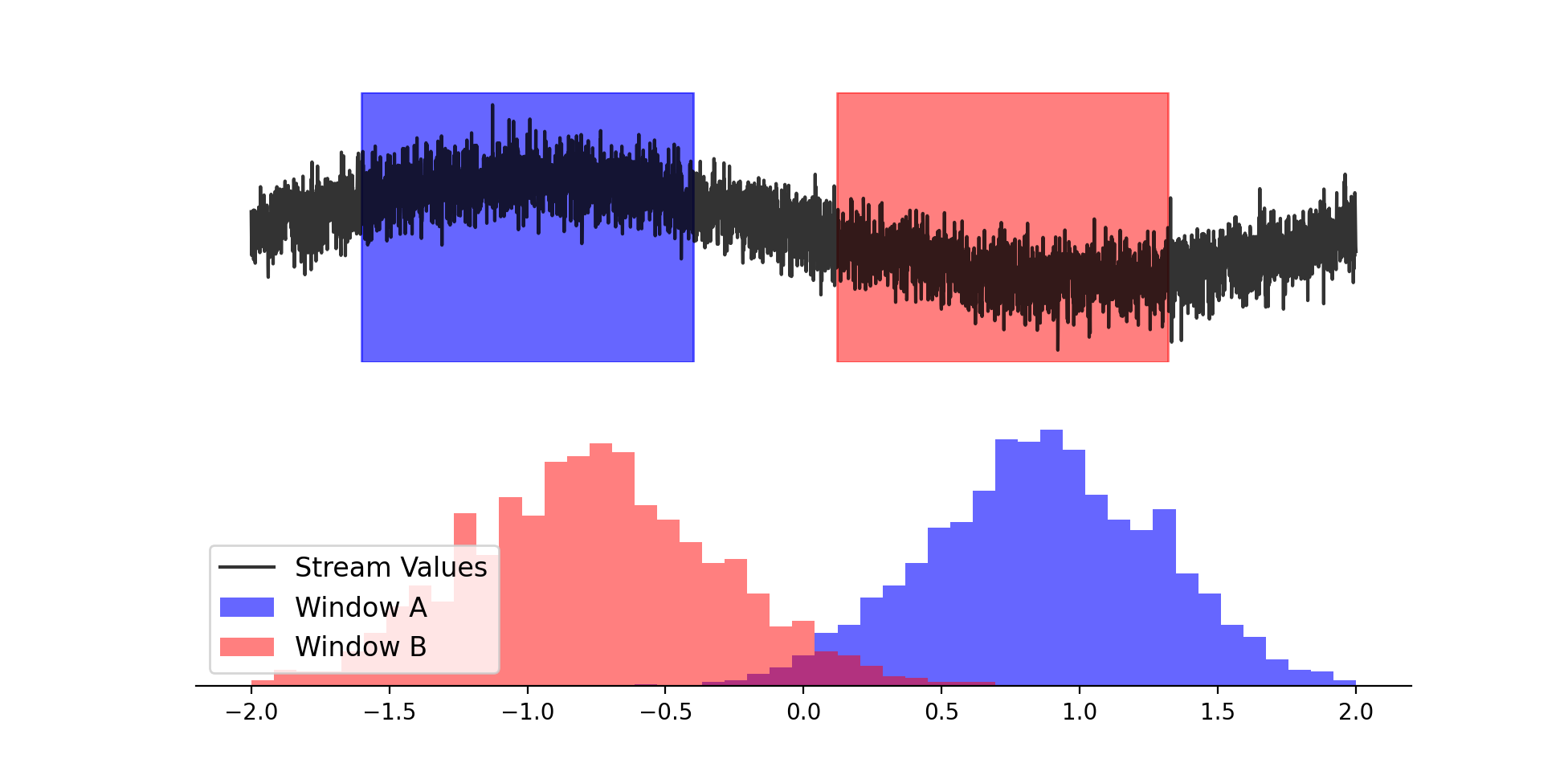
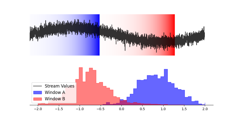
Using the formulas we derived earlier, we can implement and compare different histograms on streaming data. For a qualitative comparison, we can generate a stream where the distribution changes and compare how the methods adapt to the change in distribution.
For the graphic, we used a window size of 4000 points and a decay rate of 0.99925 (which corresponds to a 95% window size of 4000 points). It is interesting to see how the histogram outputs change in real time: by the end of the stream, the total histogram doesn’t do a very good job of capturing the distribution of values.
Finding P99 Values
We can see similar behavior if we look at percentiles. For this example, we generated a stream of exponentially distributed random variables. The exponential CDF has a clean form, so we can explicitly calculate the theoretical P99 values. We can also approximate the P99 values using our histogram implementation.
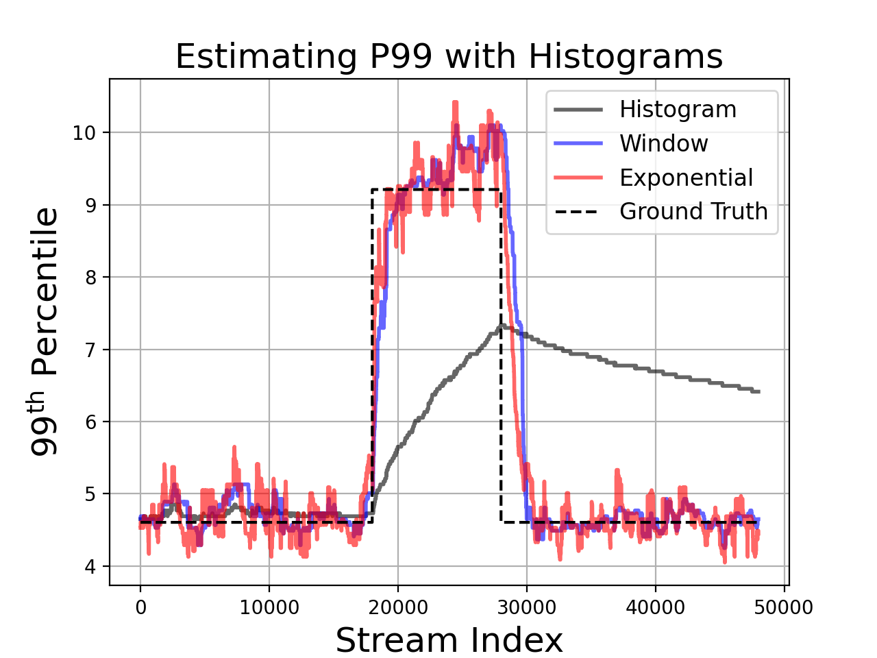
Unsurprisingly, we see that decayed histograms have lower error when the data distribution changes.
Python Implementation
Here is the streaming histogram implementation we used to compare methods. As usual, we omit the plotting code, since generating the graphics is a fairly complicated process.
import numpy as np

class StreamingHistogram():
    """A histogram for streaming data with various decay options."""
    def __init__(
            self,
            edges,
            decay = None,
            decay_rate = 0.99,
            window_size = 100):
        if decay not in [None, 'exponential', 'window']:
            raise ValueError("decay should be None, 'exponential' or "
                             "'window' but found %s." % decay)
        if len(edges) < 2:
            raise ValueError("edges should be a 1-d array-like container of "
                             "edge locations.")
        self._edges = np.sort(edges)
        self._bin_widths = np.zeros_like(edges)
        self._bin_widths[:-1] = np.diff(edges)
        self._bin_widths[-1] = self._bin_widths[-2]
        self._bin_widths[np.where(self._bin_widths==0)] = 10e-16

        self._counts = np.zeros_like(edges, dtype=float)
        self._decay = decay
        self._decay_rate = decay_rate
        self._window_size = window_size
        self._normalizer = 0
        self._buffer_idx = 0
        if decay == 'window':
            self._buffer = -1*np.ones((window_size), dtype=int)
        else:
            self._buffer = None

    def add(self, x):
        """Add value x to histogram."""
        self._decay_counts()
        # Compute index to update.
        idx = np.searchsorted(self._edges, x, side='right')
        if idx >= len(self._counts):
            idx = len(self._counts) - 1
        # Update, cache and normalize to maintain invariants.
        self._counts[idx] += 1
        self._cache_index(idx)
        self._update_normalizer()

    def pdf(self, normalize = True, density = True):
        """Return the approximate PDF (count values) from the histogram."""
        normalizer = self._normalizer
        if density:
            normalize = True  # density overrides normalize
        if not normalize or normalizer <= 0:
            normalizer = 1
        if density:
            normalizer = normalizer * self._bin_widths
        return self._counts / normalizer

    def cdf(self, normalize = True):
        """Return the approximate CDF (cumulative sum of counts)."""
        counts = self.pdf(normalize=normalize, density=False)
        return np.cumsum(counts)

    def percentile(self, p):
        """Return the bin edge corresponding to the pth percentile."""
        if p < 0 or p > 1.0:
            raise ValueError("Percentile p must be a float in [0,1], "
                             "instead got %s" % p)
        cdf = self.cdf(normalize=True)
        # we want the index corresponding to the left edge of the
        # first bin with cdf >= p.
        idx = np.searchsorted(cdf, p, side='right') - 1
        # Since np.searchsorted returns values in [0, len(edges)],
        # we only need to check the lower bound.
        if idx < 0:
            idx = 0
        return self._edges[idx]

    def clear(self):
        """Resets the histogram."""
        self._counts = np.zeros_like(self._edges, dtype=float)
        self._normalizer = 0
        self._buffer_idx = 0
        if self._decay == 'window':
            self._buffer = -1*np.ones((self._window_size), dtype=int)
        else:
            self._buffer = None

    def _cache_index(self, x):
        """Cache a previously updated index in the rotating buffer."""
        if self._buffer is not None:
            self._buffer[self._buffer_idx] = x
            # Invariant: self._buffer_idx always points to the oldest item.
            self._buffer_idx = (self._buffer_idx + 1) % self._window_size

    def _update_normalizer(self):
        if self._decay == 'exponential':
            self._normalizer = self._normalizer * self._decay_rate
            self._normalizer += 1
        elif self._decay == 'window':
            if self._normalizer < self._window_size:
                self._normalizer += 1
        elif self._decay is None:
            self._normalizer += 1

    def _decay_counts(self):
        if self._decay == 'exponential':
            self._counts = self._counts * self._decay_rate
        elif self._decay == 'window':
            delete_idx = self._buffer[self._buffer_idx]
            if delete_idx >= 0:
                self._counts[delete_idx] -= 1
Notes
-
I don’t remember who taught me this, but histograms are one of the first things to check when debugging a machine learning system. When things go wrong, it’s extremely helpful to have histograms of every possible value in the model (activations, outputs, weights, losses, etc) and the system (latencies, network transmissions, CPU load, etc). ↩
-
This is easy to show using information theory. We can do this by reduction to the INDEX problem. In the INDEX problem, Alice has a sequence of N bits x and Bob has an index n. Alice wishes to send Bob a data structure that will allow him to compute x[n]. If we have an algorithm for windowed histograms on data streams, Alice could set the window size equal to N and feed x into a histogram with two bins: 0 and 1. Bob could then stream an additional N zeros into the histogram and observe the changes in histogram bin counts to recover x. Since this process solves the INDEX problem, the histogram requires at least O(W) space. ↩