How to Find the Taylor Series of an Inverse Function

The Taylor series is a widely-used method to approximate a function, with many applications. Given a function \(y = f(x)\), we can express \(f(x)\) in terms of powers of x.

Usually, computing the Taylor series of a function is easy - just take derivatives and use the formula from an introductory calculus textbook. But what if you want the Taylor series of the function’s inverse \(f^{-1}(y)\) and you can’t write down a closed-form expression for the inverse? This is hard because we don’t have access to the derivatives any longer, so we can’t use the usual formula. But it’s still possible, and this post is going to show you how (as well as provide code to do it).

Note: If you have access to Mathematica and you just need the coefficients, try InverseSeries[Series[f]] where f is an expression for the function. Mathematica uses the series reversion technique, which works well if you only need a few terms but has disadvantages in other, more demanding situations. We’ll cover series reversion and several other methods in more detail later in the post, so stick around.

Crash Course on the Taylor Series

Eventually, we are going to build up to computing the Taylor Series of a non-analytic inverse. But before we get there, we will briefly review the Taylor series and introduce some notation.

Taylor Polynomials: Taylor polynomials are polynomials whose coefficients have been cleverly chosen to fit a function \(f(x)\) around a point \(x_0\). The n-order Taylor polynomial is as follows, where the \(c_n\) terms are called the Taylor coefficients and \(x_0\) is called the expansion point.

Taylor polynomials are useful because we can often approximate a complicated function with a low-order Taylor polynomial. The resulting approximation is typically faster to calculate and easier to analyze than the original function. To see why (and when) the Taylor polynomial is a good way to approximate \(f(x)\), we must consider the Taylor series.

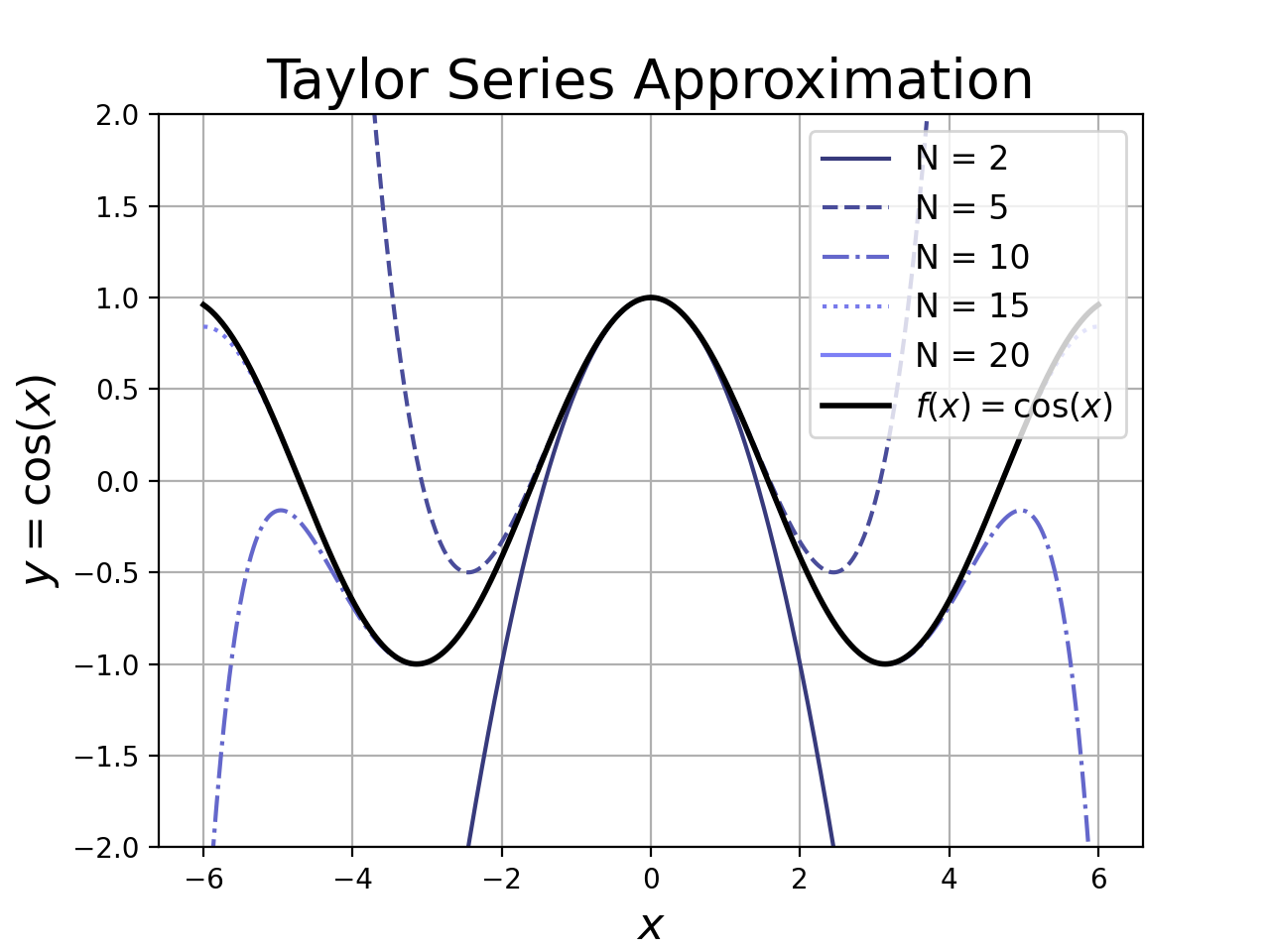
Taylor Series: The Taylor series is an infinitely-long Taylor polynomial. The nice thing about the Taylor Series is that the series converges to the function.¹

This is true for points that are near the expansion point \(x_0\). Go too far from the expansion point, and all bets are off. There are a few points that are important in practice.

1. How far is too far?

The series approximates the function for all points within the region of convergence surrounding the expansion point. The size of the region of convergence depends on the function and can range from zero to infinity. Inside the region of convergence, the Taylor series is a good approximation of the function. Outside, it might have infinite error.

2. How many terms do we need?

If the coefficients of the polynomial drop off quickly, then we can approximate the function very well using only a few terms.² This is great for applications in optimization, physics, machine learning, and pretty much everywhere else because we can approximate large / expensive functions using just a few polynomial terms. If the coefficients don’t drop off quickly, we can still do the approximation but it will require more terms.

While there are theoretical results relating the number of coefficients to the quality of the approximation, in practice we usually get the coefficients by trial and error. In fact, the vast majority of applications only go up to \(n = 1\) (linear approximation) or \(n = 2\) (quadratic approximation).

What is this good for?

The Taylor Series is an easy way to get linear / quadratic / low-order approximations of a function. These approximations are very useful and form the basis for lots of important tricks. The Taylor approximation is an essential tool for both the practitioner and theoretician alike, and it’s a major headache if you’re interested in a function that doesn’t have one.³

• Programming: Don’t want to store a lookup / interpolation table for a function like \(e^x\)? Compute the first few terms of the Taylor series until the error is smaller than machine precision.
• Physics: Don’t want to solve a non-linear differential equation? Swap out the non-linear part for a first order Taylor approximation and pray that you’re within the region of convergence.
• Engineering: Want to model an input-output relationship from lab measurements? Use least-squares to fit a Taylor series to your data, then use the Taylor model for your calculations.
• Scientific Computing: Need to add two gnarly-looking functions together? Find their Taylor series and add the coefficients.
• Optimization: Want to optimize a function with complicated gradients? Optimize over a sequence of Taylor approximations instead.
• Theory: Want to bound a complicated function with a simple polynomial? Chop off a Taylor series and bound the error with a constant. It’s also worthwhile to see if you can rearrange the Taylor series coefficients - when this works, it can result in very elegant results (see the proof of Euler’s identity).

The takeaway is that access to the Taylor series is important. If we can’t compute a Taylor series, we have fewer options for dealing with the function.

Taylor Series of an Inverse

What happens if we want to construct an approximation to \(f^{-1}(y)\)? The natural idea is to first compute the inverse of \(y = f(x)\) and then get the Taylor series. If you’re able to explicitly find \(f^{-1}(y)\), then this is clearly the best way to solve the problem.

We are interested in the case where there is no closed-form expression for \(f^{-1}(y)\). In this case, we can’t take the derivatives or use the usual methods. So how do we do it?

Series Reversion

Series reversion simplifies the problem by replacing \(f(x)\) with its Taylor series. This results in a function \(\hat{f}\) which is a good approximation of \(f(x)\). Since \(\hat{f}\) is a degree-n polynomial, we can find its inverse by solving a set of equations.

For example, if we have the (infinite) Taylor series:

And we want the Taylor series of the inverse:

We can get a system of linear equations by plugging the (unknown) Taylor series for \(f^{-1}(y)\) in for \(x\) in the first equation. This results in a rather complicated set of equations, but nonetheless yields a solution. However, there are a few drawbacks:

1. It requires that the function \(f(x)\) have a Taylor series with good convergence properties, since we need it to get the Taylor series of the inverse.
2. It requires the solution of a large set of linear equations, which can be prohibitive if we need lots of coefficients.

As a result, series reversion is appropriate for situations where we only need low-order approximations. This covers a lot of practical use cases, but there are better methods.

Lagrange Inversion Theorem

In the late 1700’s, Lagrange developed a way to directly find the expansion of \(f^{-1}(y)\) without first finding the expansion of \(y = f(x)\). This method is called the Lagrange Inversion Theorem, which I will abbreviate as the LIT. The LIT says that:

In order to put this to work in practice, we need to compute lots of derivatives for the quotient:

If \(f(x)\) has a complicated expression, this is extremely difficult to do. I say this from personal experience. I tried to apply the LIT to the research problem described at the end of the blog post, using a computer algebra system to compute the quotient derivatives. I only needed about 10 coefficients, but it took a few hours. I needed to run this computation many times, so this was unacceptable to me.

There do seem to be some new efficient methods for fast Lagrange inversion. However, I haven’t tried these techniques yet. It would be interesting to see how well it does in comparison to the following method, which I have found to be very fast.

An Efficient Recurrence Method

In a recent paper, Mikhail Itskov, Roozbeh Dargazany and Karl Hornes propose an efficient algorithm to compute the coefficients of an inverse.⁴ Rather than evaluate a complicated expression to get \(c_n\), this method recursively expresses the value of \(c_n\) in terms of previously computed coefficients.

The recursion allows the algorithm to run in a single pass and reuse many computations, which is attractive in comparison to the LIT and series reversion methods. Unlike series reversion, we don’t have to solve a big set of equations. Unlike the LIT, we don’t have to evaluate complicated quotient derivatives.

We will use the notation \(f_n\) to refer to the Nth derivative of the function.

Now, given integers \(k \ge j \ge 1\) we recursively define a set of functions \(P_{(j,k)}(x)\).

To get the expansion about a point \(y_0 = f(x_0)\), we need a “dummy variable” \(b_n\) to construct the actual coefficients \(c_n\). The procedure goes as follows.

Once we have \(b_1\), we can get the following terms using the formula:

To get the actual Taylor series coefficients, we simply divide the dummy variables by a factorial.

Note: The notation in the paper may be confusing to those coming from an engineering or science background, where the variable \(x\) often represents a continuous input variable. In this paper, it actually denotes the series coefficients! Our expression for \(c_n\) is a direct adaptation of Equation 17 in the paper, but making the appropriate subsitutions so that the formula is easier to understand.

Computing the Coefficients in Sympy

Sympy is an open-source symbolic math library for Python. It’s useful for manipulating complicated equations that would otherwise require many error-prone manual steps, so it’s perfect for computing the horrible functions \(P_{(j,k)}(x)\) from the previous section.

To start, we’ll import sympy as well as some convenience functions. If you don’t have sympy, it can be installed easily using pip install sympy. Also, let’s construct a simple function for demonstration purposes. We’ll use:

We’ll also do a much more complicated function later on.

from math import factorial
from sympy import * 

# Create the function f(x)
x = symbols('x')
fx = ln(1 + (1/x)**3)
x0 = 1.0 # expand about the point x_0 = 1
N = 20 # get first 20 coefficients

Now let’s look at what ingredients we need for the formula in the previous section. The term \(f_{l+1}(x)\) shows up in the expression for \(P_{(j,k)}(x)\), so we’re going to need the first N derivatives of \(f(x)\). We can compute them using the following Sympy code. To speed up the computations, we’ll also substitute in \(x_0 = 1\) wherever we can so that Sympy can deal with efficient floating-point values rather than its abstract representation of a function (which is less efficient).

f_n = {} # nth derivatives of f(x)
f_n_x0 = {} # nth derivatives, but evaluated at x = x_0
f_n[1] = diff(fx,x,1) # differentiate f(x)
f_n_x0[1] = f_n[1].subs({x:x0}).evalf() # do the substitution

for i in range(2,N+1):
	f_n[i] = diff(f_n[i-1],x,1) 
	# it's more efficient to differentiate the previous derivative
	# once than to directly ask for the nth derivative
	f_n_x0[i] = f_n[i].subs({x:x0}).evalf()

Now, using those derivatives, we can construct a table of all the \(P_{(j,k)}\) functions. We’ll do the same trick here so that they are immediately evaluated at \(x_0\) instead of being represented as abstract functions.

def P(N,Y): 
	# Y should contain N symbolic derivatives, where
	# Y[1] is the first derivative of f(x),
	# Y[2] is the second derivative of f(x), etc
	# 
	# Returns a hash table P: (i,j) -> symbolic equation
	# where P[(i,j)] = P(i,j) from the paper
	P = {}
	for j in range(1,N+1): 
		P[(j,j)] = Y[1]**j
		for k in range(j+1,N+1):
			P[(j,k)] = 0
			for l in reversed(range(1,k-j+1)): 
				P[(j,k)] = P[(j,k)] + (l*j - k + j + l) * Y[l+1] / factorial(l+1) * P[(j,k-l)]
			P[(j,k)] = P[(j,k)]*1/(k-j) * 1/Y[1]
	return P


P = P(N,f_n_x0) # Compute P[(i,j)] using substituted versions of f_n(x)

We’re nearly there! Now we just need to construct the coefficients from the table of \(P_{(i,j)}(x_0)\) values.

b_n = {} # Vector of pre-computed dummy variable values
b_n[1] = 1/f_n_x0[1]

c_n = {} # vector of Taylor series coefficients
c_n[1] = b_n[1] / factorial(1)

for n in range(2,N+1):

	b_n[n] = 0
	for j in range(1,n): 
		b_n[n] = b_n[n] + b_n[j]/factorial(j) * P[(j,n)]
	b_n[n] = b_n[n] * factorial(n) * -1*b_n[1]**n 
	c_n[n] = b_n[n] / factorial(n)

Note: So far, we’ve assumed that the constant term \(c_0\) is simply zero for the sake of simplicity. If this is not the case, then the solution is to put \(c_0 = f(x_0)\). This completes our calculation of Taylor series coefficients for the inverse function.

How Good is the Taylor Series?

To check whether our method works, let’s compute the Taylor approximation for the inverse function and plot the approximation against the true inverse. First, we’ll write a function to evaluate the Taylor approximation, given a set of coefficients:

def TaylorApprox(x, x0, y0, coefficients): 
	# x0: point about which we do expansion
	# coefficients: coefficient for each value n = 1, 2, ... 
	# y0: y(x0)
	# x: set of points at which to evaluate the Taylor Series approximation 
	y = np.zeros_like(x)
	for i,ci in enumerate(coefficients): 
		print(y, x, x0, ci)
		y += (x - x0)**(i+1) * float(ci)
	y += y0
	return y

Then, we’ll plot both the inverse approximation and the true inverse to see how well the two align.

import numpy as np

coeffs = [c_n[i] for i in range(1,N+1)]
y = np.linspace(0,1,1000)
y_0 = np.log(1 + (1.0/x_0)**3)
x_hat = TaylorApprox(yy, y0, x0, coeffs)

I usually don’t include the plotting code, but in this case it didn’t take much to make a nice plot.

import matplotlib.pyplot as plt

plt.figure()
plt.plot(y, x_hat, '-.', linewidth = 2, label = 'Taylor Approximation $\\widehat{f}^{-1}(y)$')
plt.plot(np.log(1 + 1/x_hat**3), x_hat, 'k-', linewidth = 2, label = 'Actual $f^{-1}(y)$')
plt.xlabel("$y$", fontsize = 16)
plt.ylabel("$x = f^{-1}(y)$", fontsize = 16)
plt.title("Taylor Series for Inverse Function",fontsize = 20)
plt.legend(fontsize = 12)
plt.grid(which = 'both')
plt.show()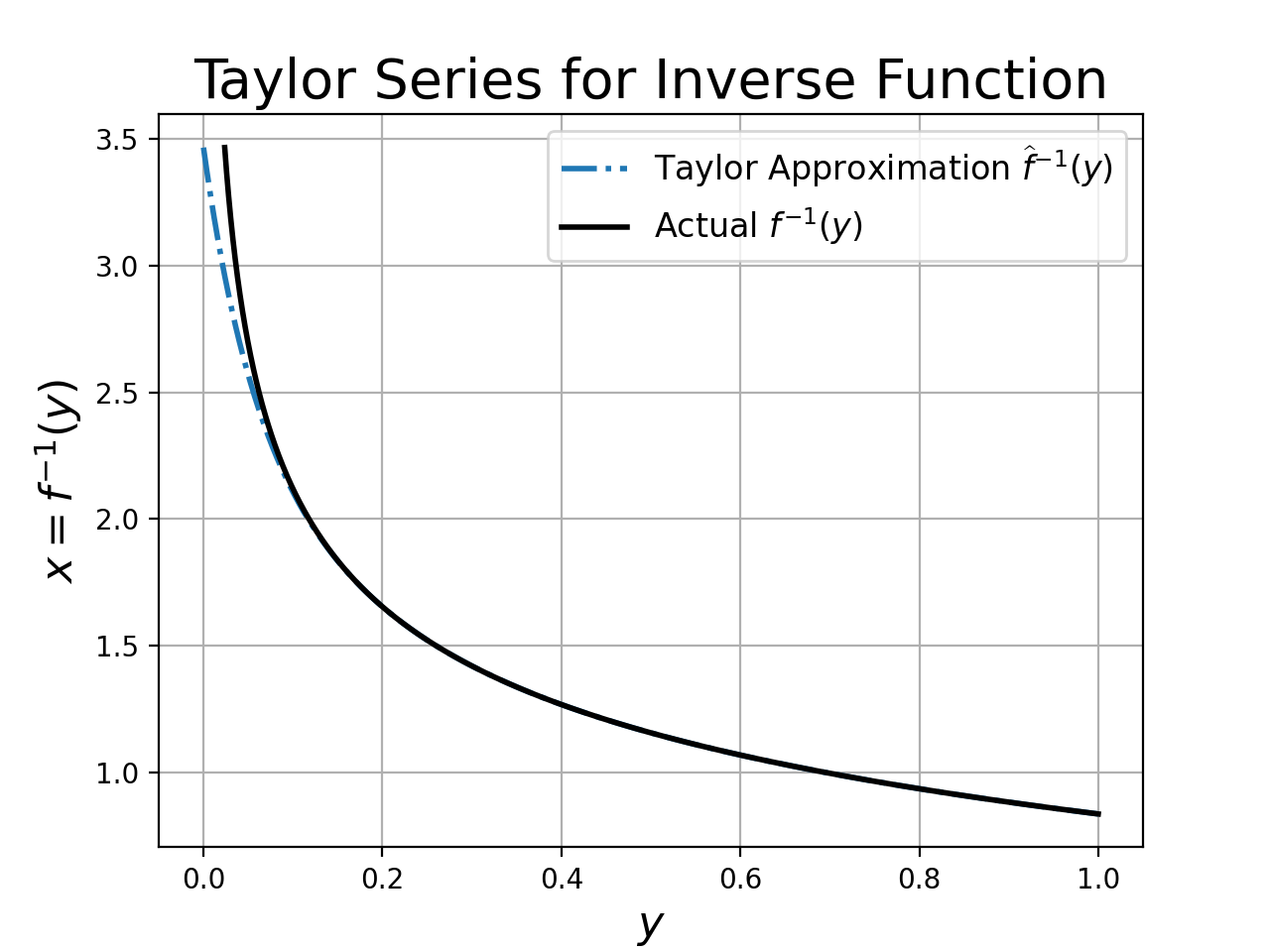

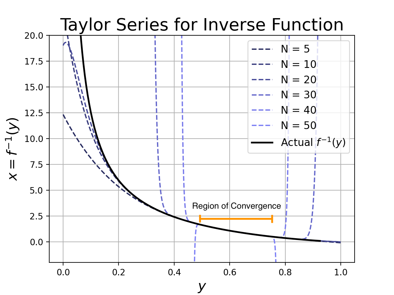
A More Difficult Example

The function that I needed to invert was more complicated than in the previous example. I wanted to invert the collision probabilities of the p-stable Euclidean and Manhattan LSH functions. This allows us to estimate the distance between two points based on their collision probability. In certain applications, the collision probability is very easy to estimate but the distance is expensive to compute.⁵ I needed the Taylor series because I wanted to triangulate the location of an unknown point by fitting a set of Taylor series coefficients to the curve generated by collisions with multiple known points on a grid.

Let’s consider the collision probability of the Manhattan LSH function. If the L1 distance between two points is \(x\), then the collision probability is:

Here, \(w\) is a parameter to the function that - for simplicity - we will set to be equal to 4 and expand about \(x = 1\). In practice, \(w\) is a tunable parameter so it was important that we be able to find the inverse easily for many choices of \(w\).

I ran the Sympy code to generate an approximation for this curve, and I obtained the following results. There are a few interesting points:

1. The recursive procedure successfully found a Taylor series for our inverse function.
2. Additional terms only improve the approximation inside a narrow region of convergence. In practice, this means that we want to use low-order approximations (at least in this case).

Sanity Check: As a final check on the code, I ran the approximation for the function \(\log(x)\) (whose inverse is the exponential function). The procedure yielded the correct coefficients.

Conclusion

We discussed methods to compute the Taylor series of an inverse function, and we presented code for one of the more recent algorithms. The method seems to work well on real problems, though we are reminded to be wary of the region of convergence when relying on high-order approximations.

Notes