Locality sensitive hashing is a super useful trick. Most people use it for near-neighbor search but it’s also helpful for sketching algorithms and high-dimensional data analysis. This post will explain four common LSH functions.
What is LSH?
Hash functions map objects to numbers, or bins. A locality sensitive hash (LSH) function \(L(x)\) tries to map similar objects to the same hash bin and dissimilar objects to different bins. The picture below shows an example where we form two hash tables - one using an LSH function \(L(x)\) and the other using a normal hash function \(H(x)\). \(L(x)\) preserves most of the clusters from the original dataset - most of the elements in each hash bin are similar. The key intuition behind LSH is that LSH functions try to group similar elements together into hash bins.

LSH collision probabilities
A hash collision occurs when two objects \(x\) and \(y\) have the same hash value. In our example, all of the red dots collided, but this was not guaranteed to happen. Under an LSH function, the chance that objects collide - called a collision probability - depends on how similar the objects are. LSH functions are defined based on their collision probabilities [1].
Definition 1: Locality Sensitive Hash Family
We say that a hash family \(\mathcal{H}\) is \((R, cR, p_1, p_2)\)-sensitive with respect to a distance function \(d(x,y)\) if for any \(h \in \mathcal{H}\) we have that
- If \(d(x,y) \leq R\) then \(\text{Pr}_{\mathcal{H}}[h(x) = h(y)] \geq p_1\)
- If \(d(x,y) \geq cR\) then \(\text{Pr}_{\mathcal{H}}[h(x) = h(y)] \leq p_2\)
The definition seems complicated, but it is really just a mathematical statement of our intuition. The picture below explains the definition. Definition 1 says that if we pick our LSH function from the hash family \(\mathcal{H}\), then all of the points in the red ball have a good chance (probability \(\geq p_1\)) of colliding with the query. All of the points in the blue shaded region have a small chance (probability \(\leq p_2\)) of colliding, and we don’t care what happens to the gray points in between.
Next, we’ll introduce LSH functions for some common distance measures. We will use \(p(x,y)\) to mean the collision probability.
1. Bit Sampling LSH
Bit sampling is one of the simplest and cheapest LSH functions. It is associated with the Hamming distance. Given two \(n\)-length bitvectors \(\mathbf{x}\) and \(\mathbf{y}\), the Hamming distance \(d(\mathbf{x},\mathbf{y})\) is the number of bits that are different between the two vectors. Bit sampling is an LSH family where
\[h_i(\mathbf{x}) = x_i \in \{0,1\}\]We choose a random index \(i\) between 0 and \(n-1\) and have the LSH function output the bit \(x_i\). To find the collision probability, observe that the number of indices for which \(x_i = y_i\) is \(n - d(\mathbf{x},\mathbf{y})\). The collision probability is simply the chance that we picked one the indices where \(x_i = y_i\).
\[p(\mathbf{x},\mathbf{y}) = 1 - \frac{d(\mathbf{x},\mathbf{y})}{n}\]2. Signed Random Projections
Signed random projections (SRP) also output binary values, but SRP is sensitive to the angular distance. To construct a SRP hash for a vector \(\mathbf{x}\), we generate a Gaussian distributed vector \(\mathbf{w}\) with the same length as \(\mathbf{x}\). The hash function is
\[h(\mathbf{x}) = \mathrm{sign}(\mathbf{w}^{\top}\mathbf{x})\]The picture shows the hash bins for a single SRP (left) and for three SRP hashes (right). This function essentially cuts the space in half and assigns points in one half to 1 and the other half to -1. The decision boundary is based on the projection vector \(\mathbf{w}\), which is orthogonal to the boundary. This function is sensitive to the angle between two vectors because if we draw a random hyperplane in \(\mathbb{R}^n\), the probability that the plane divides two points \(\mathbf{x}\) and \(\mathbf{y}\) is related to the angle \(\theta(\mathbf{x},\mathbf{y})\).
\[p(\mathbf{x},\mathbf{y}) = 1 - \frac{\theta(\mathbf{x},\mathbf{y})}{\pi}\]The picture below provides intuition for why SRP is sensitive to angles. The probability that \(h(\mathbf{x}) \neq h(\mathbf{y})\) is the probability that a randomly chosen line falls between \(\mathbf{x}\) and \(\mathbf{y}\). If we randomly pick an angle, there is a \(\frac{\theta}{\pi}\) chance that it falls between the two points and separates them.
This hash function can be very fast, especially when we use sparse random projections. For more information, see [2,3].
3. Euclidean and Manhattan LSH
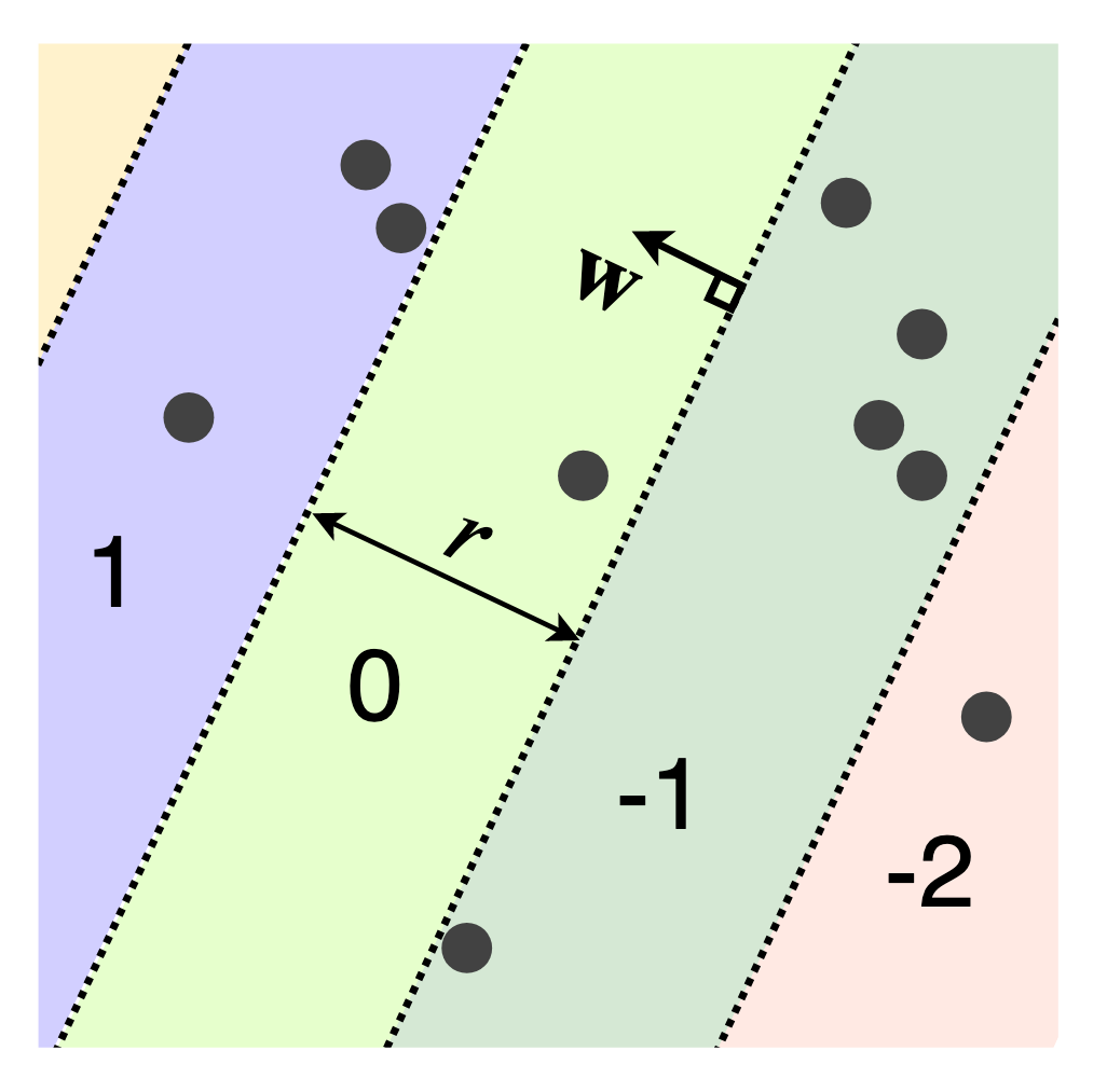
The LSH functions for the Euclidean (L2) and Manhattan (L1) distances are also based on random projections that cut \(\mathbb{R}^n\) into pieces [4]. Each piece becomes a hash bin. The hash function is identical to SRP, but we round instead of taking the sign of the projection. This produces hash bins that repeat in the direction of \(\mathbf{w}\) instead of a single decision boundary as with SRP.
\[h(\mathbf{x}) = \Big\lfloor \frac{\mathbf{w}^{\top}\mathbf{x} + b}{r}\Big\rfloor\]The user-defined parameter \(r\) determines the width of each hash bin, and \(b\) is a random number in the range \([0,r]\). If we generate \(\mathbf{w}\) with a Gaussian distribution, we get an LSH function for the Euclidean distance, while a Cauchy distribution results in an LSH for the Manhattan distance. Unlike the previous LSH functions, this hash function maps to the entire set of integers. The analytic expression for the collision probability is complicated to write down but a closed-form expression is available in [4].
4. Clustering LSH
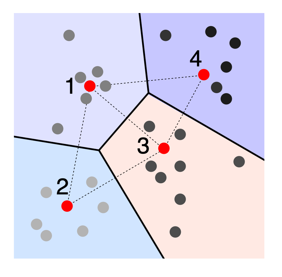
Clustering LSH is an example of a learned or data-dependent LSH function. The idea is to find a set of cluster centers \(\mathcal{C}\) that do a good job of approximating the dataset, shown in red. These centers might be found using k-means clustering, convex clustering, or any other clustering method. We can also select cluster centers randomly or on a grid, but we might need a larger number for good performance. Once we have the cluster centers, we assign an integer value to each one. The hash bins for \(h(x)\) are the same as the Voronoi cells for the set of centroids. Given an object to hash, we find the nearest center and output its index.
\[h(x) =\underset{1 \leq i \leq |\mathcal{C}|}{\mathrm{arg\,min\:}} d(x,c_i)\]It is easy to show that this function is locality-sensitive but much harder to specify the collision probability, since collisions depend on the set of learned cluster centers \(\mathcal{C}\).
References
[1] Indyk, P., & Motwani, R. (1998, May). Approximate nearest neighbors: towards removing the curse of dimensionality. In Proceedings of the thirtieth annual ACM symposium on Theory of computing (pp. 604-613). ACM.
[2] Li, P., Hastie, T. J., & Church, K. W. (2006, August). Very sparse random projections. In Proceedings of the 12th ACM SIGKDD International Conference on Knowledge Discovery and Data Mining (pp. 287-296). ACM.
[3] Achlioptas, D. (2001, May). Database-friendly random projections. In Proceedings of the twentieth ACM SIGMOD-SIGACT-SIGART symposium on Principles of database systems (pp. 274-281). ACM.
[4] Datar, M., Immorlica, N., Indyk, P., & Mirrokni, V. S. (2004, June). Locality-sensitive hashing scheme based on p-stable distributions. In Proceedings of the twentieth annual symposium on Computational geometry (pp. 253-262). ACM.
[Photo Credit] Jeremy Bishop on Unsplash