Streaming Algorithms for Discrepancy Minimization

Minimizing discrepancy is a core part of several recent proposals for efficient machine learning and dataset summarization. Unfortunately, the problem is NP hard, and we are forced to use approximate solutions.

Some of these approximations are expensive, but they don’t have to be. Thanks to new research on the problem, we can now do a reasonably good job in a single pass through the data.

This post is aimed at practitioners who want to try out machine learning algorithms involving discrepancy but don’t want to solve hard optimization problems to do it. I’ll talk about two recent methods that I’ve used with good success. The algorithms are fast even for million-scale datasets, are super simple and can be implemented in under 10 lines of Python.

Discrepancy Minimization Problem

We’re going to consider the following discrepancy minimization problem:

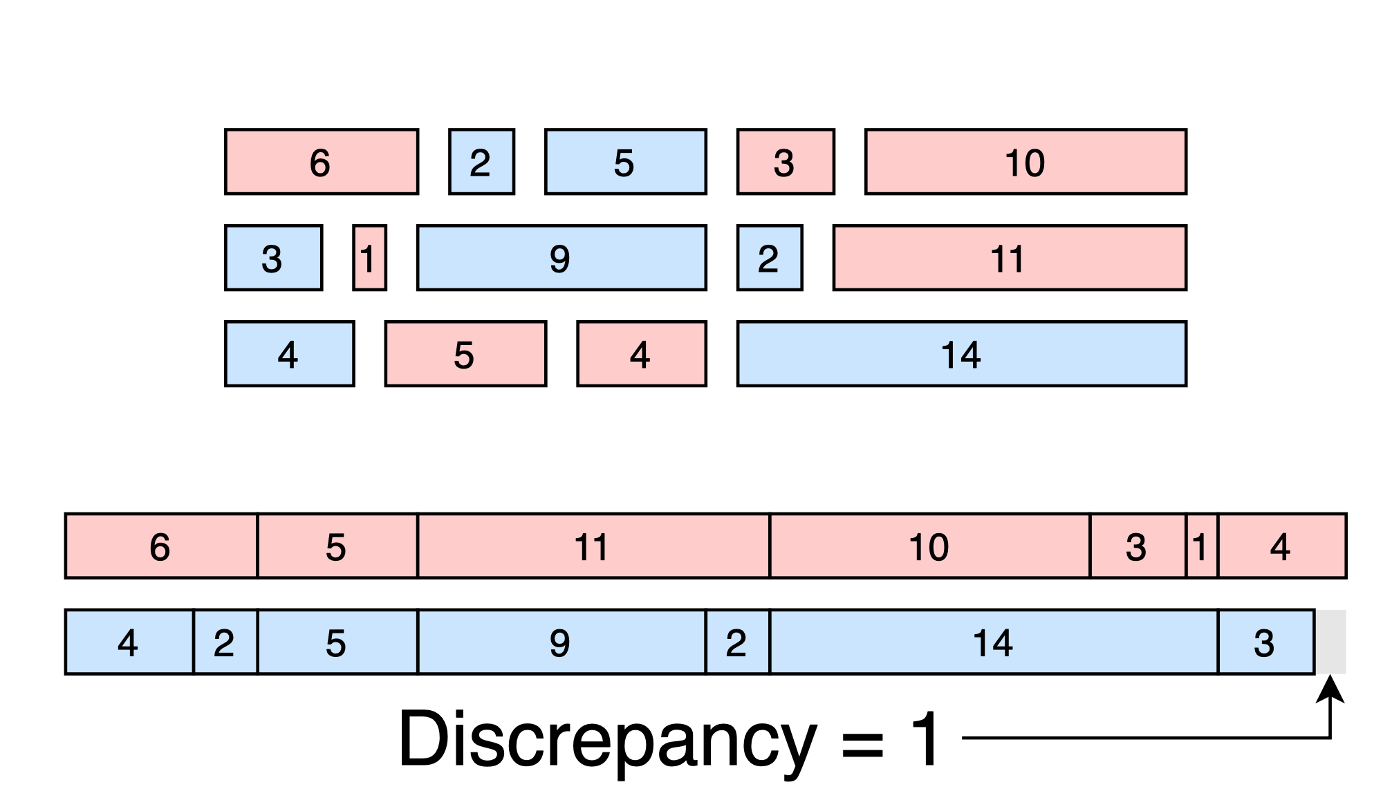
Discrepancy Minimization: Given a set of d-dimensional vectors \(x_1, x_2, ... x_N\), choose signs \(s_1, s_2, ... s_N\) to minimize the discrepancy:

In other words, we want to break the set of N points into two optimally balanced groups - one with sign +1 and the other with sign -1.

Discrepancy for Machine Learning

This idea of discrepancy is different from the one that’s used in the construction of coresets, loss estimators, fast neural networks and other machine learning applications. In machine learning, we actually care about how the groups differ in terms of the loss for a model \(\theta\).

However, the two ideas are closely related. In practice, I’ve found that the mismatch doesn’t really matter - you get roughly the same results.

For models where the loss is a function of the inner product \(\langle x_n, \theta\rangle\), you can make this relationship explicit by looking at the Taylor expansion of the loss function. If you’re interested, see Lemma 17 of this paper.

Discrepancy Minimization via a Self-Balancing Walk

Alweiss, Liu and Sawhney published a paper in STOC 2021 that directly addresses the streaming discrepancy problem.¹ Their randomized algorithm comes with strong theoretical guarantees and (to my knowledge) is the first to rigorously solve the problem in \(O(N)\) time.

What’s more, their method is extremely easy to implement. This is a pleasant surprise, since algorithms presented at STOC and FOCS aren’t always easy to translate to practice.² Here is an implementation in Python.

def discrepancy_ALS(dataset, failure_rate = 0.1):
	# Dataset is a (N,d) array-like of floats
	# failure_rate is the probability that we will
	# not find a solution with low discrepancy
	# (in practice, this can safely be set to 10%)
	N = dataset.shape[0] # number of entries
	d = dataset.shape[1] # number of dimensions 
	signs = [] # output
	w = np.zeros_like(dataset[0],dtype=float)
	c = 30*np.log(N*d/failure_rate) # constant
	for x in dataset:
		prob = 0.5 - np.dot(w, x)/(2*c)
		z = np.random.random()
		if z > prob:
			sign = -1
		else:
			sign = 1
		signs.append(sign)
		w = w + sign*x

	# compute overall discrepancy
	disc = np.zeros_like(dataset[0], dtype=float)
	for x, sign in zip(dataset, signs):
		disc += x * sign
	return (signs, np.max(np.abs(disc)))

Explanation of the Algorithm

The algorithm uses a “memory vector” \(w\) that remembers the running totals for each dimension. We want each dimension of the memory vector to be as close to zero as possible. If the discrepancy starts to get too big for a particular dimension, the corresponding entry of \(w\) will be large as well. We use this information to pick a sign that will push \(w\) back towards zero - in other words, we use a self-balancing random walk.

Better Practical Results with Heuristics

The previous algorithm works well and is efficient, but the large value of c causes it to frequently pick the same sign early in the algorithm. I learned from Tung Mai and Anup Rao³ that good heuristic is to simply set c = 1.

Unfortunately, this breaks the theoretical analysis in ways that seem difficult to fix. There is a paper describing the heuristic, but the theoretical issues remain open.

def discrepancy_ADMR(dataset):
	# Dataset is a (N,d) array-like of floats
	signs = [] # output
	w = np.zeros_like(dataset[0],dtype=float)
	for x in dataset:
		prob = 0.5 - np.dot(w, x)
		prob = 0 if prob < 0 else prob
		prob = 1 if prob > 1 else prob
		z = np.random.random()
		if z > prob:
			sign = -1
		else:
			sign = 1
		signs.append(sign)
		w = w + sign*x

	# compute overall discrepancy
	disc = np.zeros_like(dataset[0], dtype=float)
	for x, sign in zip(dataset, signs):
		disc += x * sign
	return (signs, np.max(np.abs(disc)))

The algorithm is exactly the same as before, but now we do not have to know the number of items, N, in the data stream. We also don’t have to set the failure probability. Overall, this version is practically much more useful because the user does not have to set any parameters.

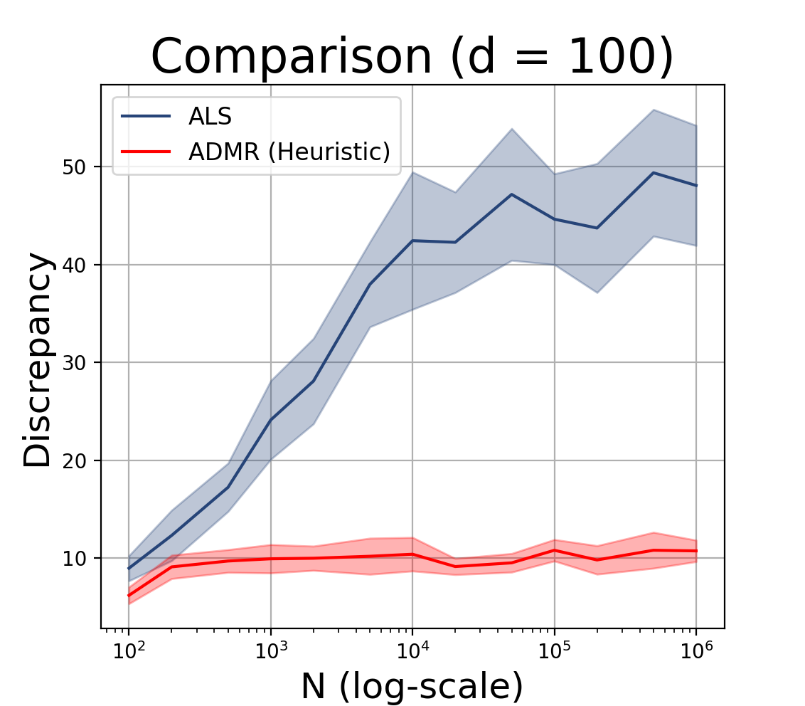
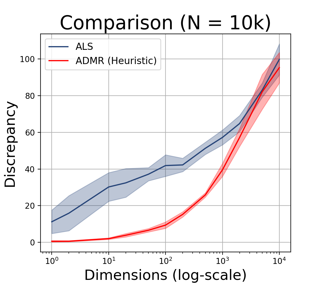
Experimental Comparison

To see how well the algorithms do, I ran them on problems of varying size and dimension. As the input, I used N random points inside the d-dimensional unit hypercube. As the output, I measured the discrepancy found by the algorithm (lower is better). I report the mean and standard deviation over 10 experiments, where the randomness is over both the algorithm and the uniformly sampled dataset.

Theoretical Guarantees

This section is not terribly important from a practical perspective, but it’s interesting and possibly useful (if you’re using these algorithms as a building block for other applications). The theoretical objective is to prove that the signs chosen by the algorithm result in low discrepancy.

Given any set of N vectors, the lower bound for the problem is at least:

This means that no matter what algorithm we pick, there will always be adversarial problem instances where we cannot get smaller than (roughly) \(\log N\) discrepancy. The algorithm from STOC 2021 has discrepancy:

where \(\delta\) is the failure rate. The streaming algorithm is fairly close to optimal - only a factor of \(\sqrt{\log N}\) away. The heuristic doesn’t have any guarantees, but it works better in practice. I suspect that for specialized problem instances, there are other heuristics that work even better. It would be interesting to see if provable statements can be made about the heuristic methods if we restrict our attention to specific problem instances, such as uniform or Gaussian distributions for x.

Conclusion

Discrepancy minimization is a core subroutine in a number of recent algorithms in machine learning. For example, coresets often involve some kind of discrepancy-minimizing partition. We introduced two efficient ways to solve this problem that work on streaming data and don’t need lots of RAM. If you encounter a use case for discrepancy minimization, consider using one of the methods.

Notes