Streaming Coresets with Discrepancy Minimization

Edo Liberty and Zohar Karnin introduced a new way to construct coresets for many problems in a recent COLT paper. Their algorithm is interesting because it departs from well-established ways to construct coresets. Most coreset constructions are based on (approximate) importance sampling and sensitivity scores. Theirs is based on dividing the dataset into pieces to satisfy a discrepancy criterion.

In this post, I’ll break down their ideas in an easy-to-understand way and explain why I think this is interesting.¹

What is a Coreset?

Suppose we are given a dataset of N points \(D = \{x_1, x_2, ... x_N\}\). A coreset is a “core set” of points that do a good job of summarizing the dataset for a particular task.

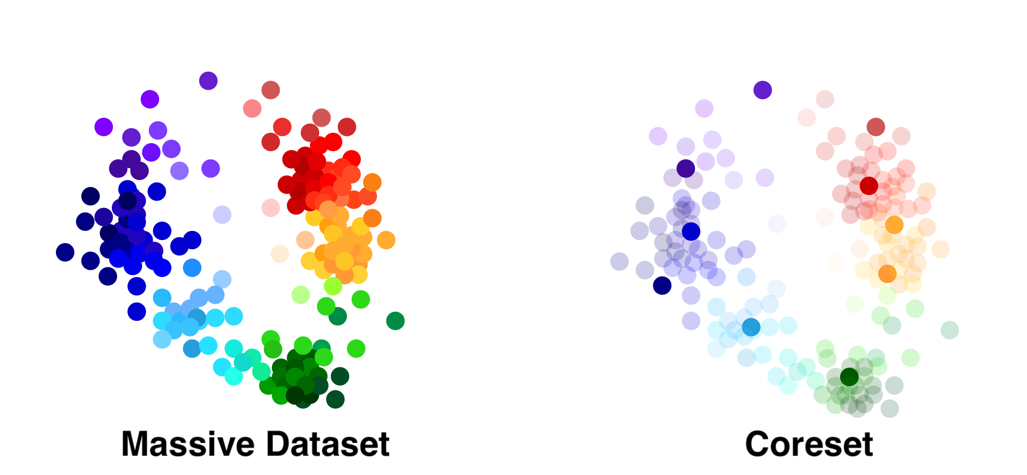
The coreset in the picture consists of the dark points (right), which were selected from the full dataset (left). The paper considers coresets with an additive error guarantee. Given a function \(f(x,q)\), an additive coreset is a set of points and weights \(C = \{(z_1,w_1),...(z_M,w_M)\}\) such that

\[|\sum_{x\in D} f(x,q) - \sum_{(z,w) \in C} w f(z,q)|\leq N \epsilon\]

In other words, we bound the error of the difference between the sum of functions on the coreset and the sum over the original dataset.² To understand the practical meaning of this guarantee, suppose that \(f(x,q)\) is a loss function for a machine learning model. The input \(x\) is a data point from our dataset and the query \(q\) is a set of model parameters.

What is Discrepancy?

Discrepancy is a measure of redundancy in a dataset. To explain discrepancy, we’ll begin with a really simple problem. It might not seem relevant at first, but we’ll use this problem to build up to an understanding of discrepancy-based coresets. The problem goes like this:

Say we have a set of numbers \(y = [y_1, y_2, ... y_N]\). Our job is to partition the numbers into two groups so that the numbers in each group add to the same value.

Of course, this might be impossible - it might be that no matter how we split the numbers, we can’t separate them into two perfectly-balanced groups. In that case, we’ll settle for two nearly-balanced groups, where the sums are nearly the same.

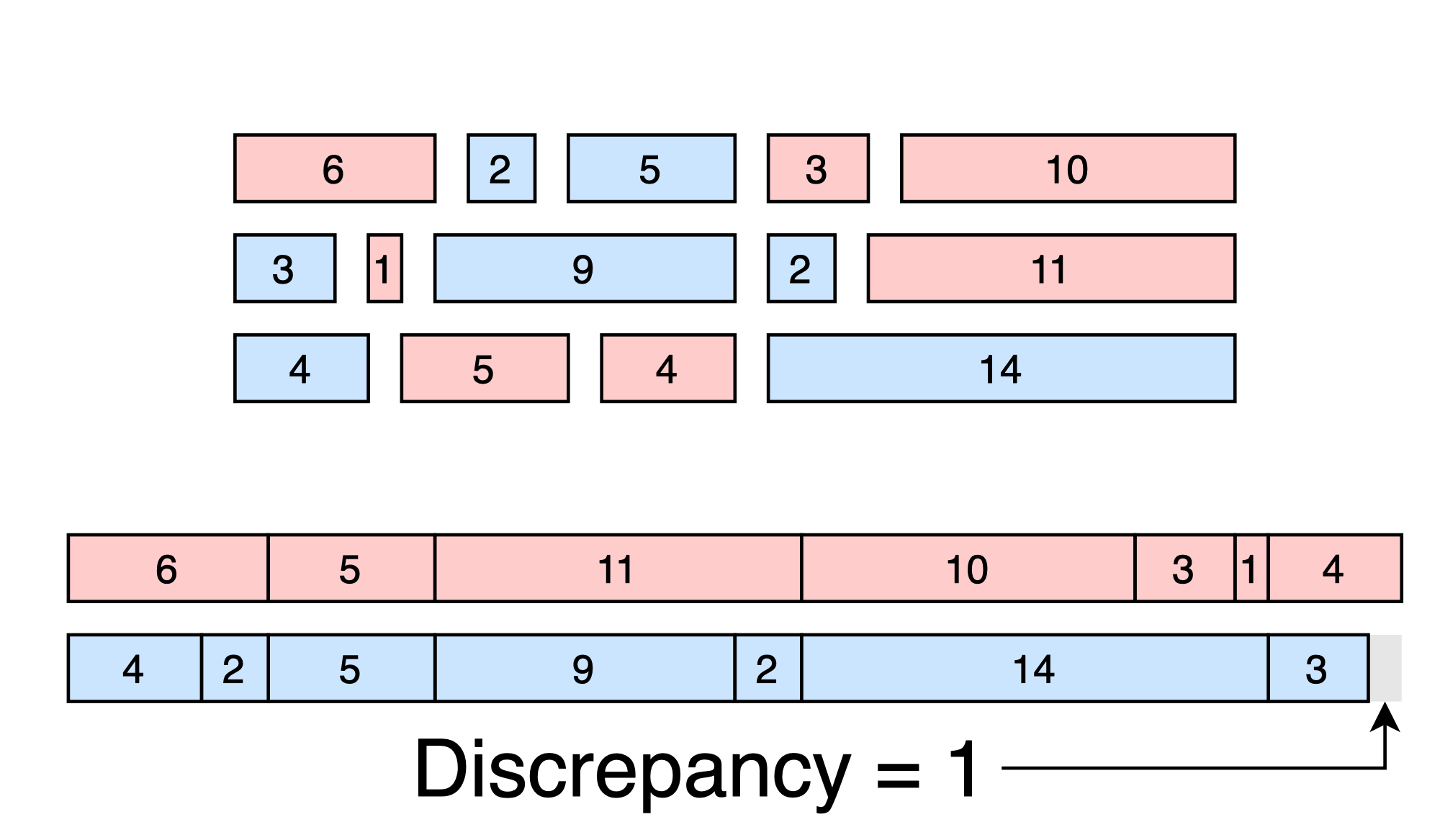
The discrepancy is the size of the difference between the sums. If we can perfectly balance the groups, then the discrepancy is zero. If the groups are nearly balanced, then the discrepancy is small. Thus, discrepancy measures the dissimilarity between the groups - low discrepancy means that the two groups contain the same information (at least in aggregate).

Optimizing for Discrepancy

How can we optimize the groups to minimize discrepancy? Let’s examine a simple objective function that measures the difference between the sums.

\[F(G_1, G_2) = \left|\sum_{y_i \in G_1} y_i - \sum_{y_i \in G_2} y_i\right|\]

The interesting part of this expression is that we can re-write it as a sum over all the numbers, multiplied by a sign vector \(s \in \{+1,-1\}^N\). Entry \(i\) of the sign vector is positive if the corresponding number \(y_i\) is in the first group; otherwise it’s negative.

\[\mathrm{Discrepancy}(s) = \left|\sum_{i = 1}^N s_i y_i\right|\]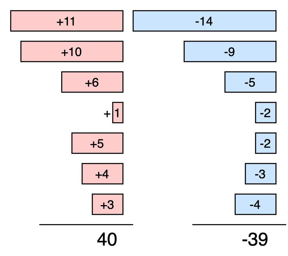

We have reduced the group assignment problem to finding an N-dimensional sign vector (which is easier to deal with mathematically). Once we have the sign vector, it’s easy to partition points into low-discrepancy groups by simply collecting all points with the same sign.

\[s^{\star} = \underset{s}{\mathrm{arg\,min}} \left|\sum_{i = 1}^N s_i y_i\right|\]

Notes: Without making assumptions about the distribution of numbers, this problem is NP-hard.³ This shouldn’t come as a surprise - problems involving the assignment of elements to groups to maximize a global objective are usually difficult. We will take the pragmatic approach and refuse to worry about NP-hardness until it becomes a problem.⁴ Also, note that some authors write the discrepancy with a \(1/N\) term (i.e. the average rather than the sum). This does not affect the results in any way.

From Discrepancy to Coresets

What if we wanted to efficiently estimate the sum of the entries of \(y\) without computing all N terms of the sum? This is a little pointless, since it’s not all that expensive to compute a sum over N scalars, but it’ll help set up the problem for later. Since the groups are disjoint, we can break the overall sum into two sums - one within each group.

\[\sum_{i = 1}^N y_i = \sum_{y_i \in G_1} y_i + \sum_{y_i \in G_2} y_i\]

If we have a well-balanced grouping, we know that the sum over \(G_1\) is approximately equal to the sum over \(G_2\). Remember from before that the discrepancy is the difference between the sums. If our grouping has low discrepancy, then we can efficiently estimate the overall sum.

Why? Suppose that the discrepancy is less than \(\Delta\). That means that the sums over \(G_1\) and over \(G_2\) are within \(\Delta\) of each other:

\[\sum_{y_i \in G_1}y_i - \Delta \leq \sum_{y_i \in G_2} y_i \leq \sum_{y_i \in G_1} y_i + \Delta\]

In other words, we only need to compute one of the sums! We can approximate the second sum using the one we’ve already computed, introducing at most \(\Delta\) error. In other words, we can estimate the overall sum as:

\[\sum_{i = 1}^N y_i \approx 2 \sum_{y_i \in G_1} y_i\]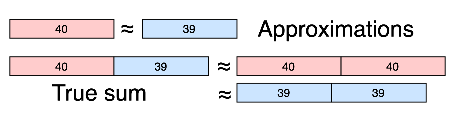

A few observations:

• Each group is a \(\Delta\)-additive coreset for the sum. We can pick either one.
• We pick the smaller of the two groups when computing the sum, to minimize the number of calculations.
• Since we partitioned N points into 2 groups, the smaller group is never larger than \(N/2\).
• The error of the final estimate is the discrepancy between the groups.

Maximum Discrepancy

By now, it should be clear that - given a low-discrepancy grouping - we can efficiently approximate sums by restricting our attention to one of the groups. How can we extend this idea to work for pairwise sums?

The most glaring issue is that we are no longer dealing with a single set of numbers \(y = [y_1, ... y_N]\). Instead, our set depends on the query \(q\).

\[y = [f(q, x_1), f(q, x_2), ... f(q, x_N)]\]

Likewise, the discrepancy also depends on \(q\).

\[\mathrm{Discrepancy}(s) = \left|\sum_{i = 1}^N s_i f(q, x_i)\right|\]

This is a problem because we need the grouping to be low-discrepancy no matter what query we pick. There could be an unlimited number of queries, so it’s unreasonable to check the discrepancy for every one of them.

The solution is to optimize the grouping over the worst case discrepancy. This amounts to minimizing the maximum discrepancy, where the maximum is taken over all possible queries.

\[s^{\star} = \underset{s}{\mathrm{arg\,min}} \left( \underset{q}{\max} \left|\sum_{i=1}^N s_i f(q,x_i)\right|\right)\]

This seems difficult because the maximum discrepancy could be really large - maybe there is a pathological query somewhere that makes the problem hard. But for many problems, we can bound the discrepancy for any query and any set of points.

For example, if \(f(q,x)\) is a logistic regression model in \(d\)-dimensional space (\(d\) features), then

\[\underset{q}{\max} \left|\sum_{i=1}^N s_i f(q,x_i)\right| \leq O(N\sqrt{d})\]

There are many other examples (sigmoid activation, Gaussian kernel, etc). Because we can find a low-discrepancy assignment for these problems, we can construct coresets to solve them. This is the central observation of the paper by Karnin and Liberty.

The Coreset Algorithm

The simplest way to turn this idea into a coreset is to solve the max-discrepancy problem over the complete dataset. Suppose we have an algorithm that can process a set of \(N\) input points to obtain a grouping with max-discrepancy \(\leq \Delta N\). If we run this algorithm over a dataset with \(N\) points, then we get a set of (at most) \(N/2\) output points, each having a weight equal to 2. The error of the coreset is \(\leq \Delta N\).

If we want a smaller coreset, we can run the max-discrepancy algorithm again over the \(N/2\) points to get a set of \(N/4\) points with weight equal to 4 and error \(\leq 2 \Delta N\).

To see why, think of the discrepancy minimization algorithm as a black box. We feed the algorithm \(N/2\) points and get out \(N/4\) points. If the \(N/2\) input points had a weight of 1, then the error over the output points would have been \(\leq \Delta N/2\). But because they actually have a weight of 2, the error gets multiplied by 2 as well, resulting in error \(\leq \Delta N\).

This error is between the \(N/4\) point approximation and the \(N/2\) point approximation, but remember that the \(N/2\) points are themselves an approximation of the full dataset. So, this error adds to the original error from the previous step.

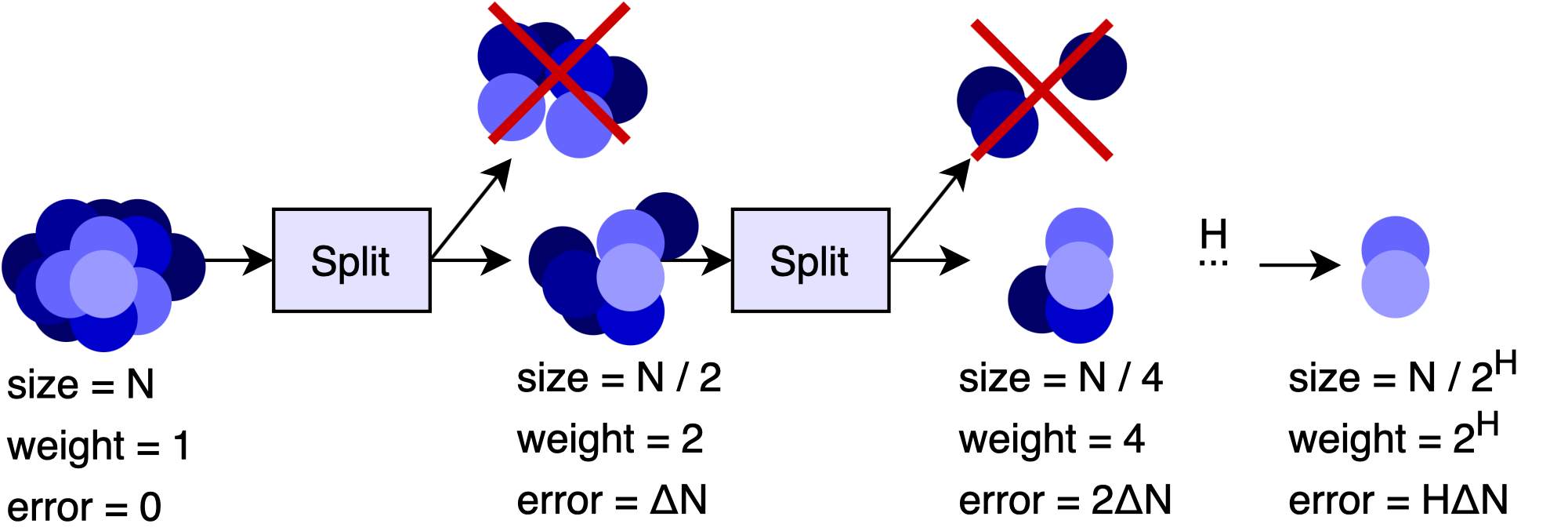
We aren’t limited to just two runs - we can keep re-running the algorithm until we have a very small set of points. If we run the algorithm \(H\) times, we get \(\frac{N}{2^H}\) points with weight \(2^H\) and error \(H \Delta N\). In other words, we have an \((H \Delta)\)-additive coreset.

Why is this a good coreset?

Let’s take a look at the relationship between the number of points and the error. With \(\frac{N}{2^H}\) points, we get \(H \Delta N\) error. An exponential decrease in the number of points leads to a linear increase in the error! This is fantastic because we can dramatically reduce the size of the coreset without substantially increasing the error.

Another attractive feature is that all of the weights are the same. This is good if we want to train a neural network or using the coreset. There’s recent evidence to suggest that large weight deviations lead to problems with SGD and optimization. Unlike other coreset methods, the discrepancy technique does not suffer from these problems because all the weights are the same. To the best of my knowledge, this is the only kind of coreset with this property.

Streaming Version

In big data problems, we often don’t have enough computational resources to store or process all of the points at once. This can be formalized using the data streaming model. In the streaming setting, we see each data point one at a time. We’re allowed a small amount of memory relative to the total number of points (typically logarithmic in the stream size), and we’re asked to come close to the true solution.

Some discrepancy minimization algorithms can work in the streaming setting, but most need to see the full point set. We can’t directly use these methods. But once again, Karnin and Liberty provide a clever solution - this time in the form of a multi-level system of buffers. The idea is that each buffer collects items until it is full. Once this happens, the buffer computes a low-discrepancy partitioning over its points and throws away one of the two resulting groups.⁵ Each buffer in the chain is called a compactor. Just as a soil compactor squeezes rock into a small cube of gravel, the discrepancy compactor squeezes the elements in the buffer into a small output subset. It’s not a perfect metaphor, but it’s still a good name.

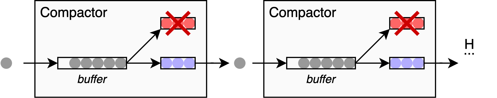
The overall error is the sum of discrepancies from each step, and it is not too much larger than the offline error. See the paper for details.

Why is this interesting?

I think discrepancy is an interesting tool for constructing coresets because it selects points in a way that is fundamentally different from other construction methods.

Most coresets are constructed using importance sampling. To briefly explain this technique, we start by assigning an “importance” to each point in the dataset. Then, we randomly select points to include in the coreset based on their importance. The higher a point’s importance, the more likely it will be included. The result is a coreset composed of the most important points from the dataset.

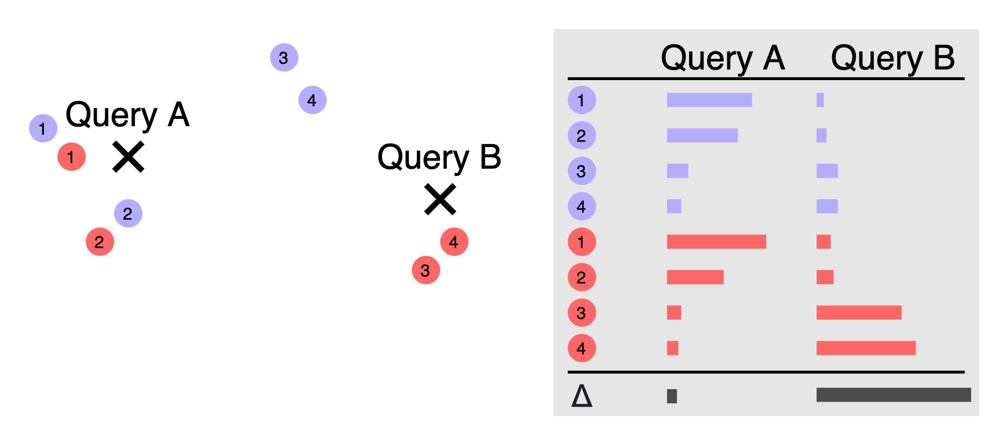
Discrepancy is different - it eliminates points based on redundancy. Discrepancy tries to balance the points so that the two groups cancel out in the sum. If we have points with similar contributions, they will probably get sent to opposite groups. This happens when points \(x_1\) and \(x_2\) induce similarly-shaped loss functions \(f(q,x_1)\) and \(f(q,x_2)\). As a result, discrepancy is conceptually not so different from \(k\)-means clustering. It prunes points based on whether the group already has something similar.

To understand the difference between importance and redundancy, think about what happens when we have two identical points in the dataset. For sensitivity sampling, the importance of a point depends on two things:

1. The number of similar points
2. The maximum contribution of the point to the sum

Most importantly, identical points have the same importance weights. If we use importance sampling, we will correctly identify whether the points are important, but we might accidentally sample both of them. This is clearly a waste, since we could’ve gotten a smaller coreset by keeping one of the points and assigning it a weight of two.

On the other hand, the discrepancy method will assign the points to opposite groups (and therefore only keep one of them). This happens because the contributions of each point will perfectly cancel each other out if the two points are assigned opposite signs. The discrepancy method has identified that the second point is redundant and has discarded it.

Conclusion

Discrepancy is an interesting mechanism for downsampling large datasets. From a theoretical perspective, it seems to compress data much differently than well-established techniques based on sensitivity sampling. There are also practical advantages. Discrepancy is straightforward to implement, works in the streaming setting, and produces coresets with near-uniform weights. I would be strongly interested to see how this approach works for real problems.

Extensions

We could take the idea in a few interesting directions. I am not sure whether there is room for theoretical improvement, since coresets have well-known lower bounds. However, there might be some tricks to get good practical performance with a smaller coreset size on many important problems.

One direction is to minimize the maximum discrepancy over a limited set of queries. We might be able to improve performance by preserving the error guarantees only for reasonable queries rather than for all possible queries. This idea could have practical consequences for empirical risk minimization, where we only care about the error for models that are close to the optimum. It would change the optimization problem, possibly even making it easier. For example, if the query set is a ball and the function is smooth, then we likely only need to enforce the discrepancy condition at the center of the ball.

Another interesting idea is to combine the importance sampling and discrepancy approaches. The strength of discrepancy sampling is that it can reduce the redundancy of the dataset. The strength of importance sampling is that it can ignore irrelevant information. The two methods seem to have complimentary strengths and weaknesses, so a combination might work well. For example, one could construct a coreset using a chain of compactors that alternate between discrepancy and importance sampling. Since discrepancy has additive guarantees and sensitivity has multiplicative guarantees, this method might satisfy the definition of a weak coreset, which uses a combination of additive and multiplicative errors.

---