A Zoo of Near Neighbor Problems

There are too many near neighbor problem statements. There. I said it. When I first tried to read about this, it took me forever to understand all the different ways to formalize the same problem.

It took me even longer to understand why we have so many near neighbor problem statements, all of which are slightly different. I think the main reason is that the natural formulation of the problem is hard, leading to many relaxations. Also, everyone has a different reason to do near neighbor search. A relaxation that makes sense in one context does not necessarily make sense in another one.

For example, people who work on natural language processing and recommender systems often embed objects as high-dimensional vectors. Similar objects have nearby vectors, and the first stage of information retrieval often amounts to finding a big set of embeddings that are close to a query. In this case, does it matter whether we get all of the nearest neighbors correct? Probably not, especially since the top \(K\) elements will usually get re-ranked later anyway. But if we had a nearest neighbor classifier, we might make the wrong classification decision near the boundary of two classes. In this case, an approximate answer might not be any good.

This post presents a reasonably complete set of near-neighbor problems, along with some recent extensions and assumptions. Since our purpose is to develop intuition, the problems are described very informally - please refer to the published literature if you want rigorous and explicit problem statements.

99 Problem Statements

Given an \(N\)-point dataset \(D\) that consists of vectors \(x \in \mathbb{R}^{d}\), our job is to find a set of points from \(D\) that are close to a query \(q\). This is a simple idea, but there are nearly a dozen different ways to formalize the problem. Conceptually, the simplest idea is to just return the nearest points.

K-Nearest Neighbor (KNN): Return the \(k\) nearest points from \(D\) (i.e. those with the smallest \(\mathrm{dist}(x,q)\))

Unfortunately, exact solutions scale poorly with the dimensionality, and we inevitably need to do an exhaustive search that handles all edge cases. There isn’t enough flexibility in the problem statement to allow fast solutions, so the theory community developed multiple relaxations of the problem.

Relaxations

How could we go about relaxing the nearest neighbor problem? We could simply allow a few of the top \(K\) entries to be incorrect, as if we’d randomly replaced some of the top neighbors with different points. But the randomized version of the exact KNN problem is asymptotically no easier than the original problem,¹ so we need to adjust the problem in a different way. One way is to allow some “wiggle room” in the distance between the neighbors and the query.

c-Approximate K-Nearest Neighbor (C-KNN): Solve the KNN problem, but it’s okay if you return a point within \(C\) times the distance from the query to the \(i\)-th nearest neighbor instead of the exact \(i\)-th nearest neighbor.

It turns out that for many algorithms, the hardness of search strongly depends on the distance between the query and the neighbors.² The search is easiest when the neighbors are close to the query, but harder when the neighbors are at a greater distance. This behavior means that any variation of the KNN problem (including C-KNN) is coupled in deep and unpleasant ways with the dataset and query.

For example, the nearest \(K\) points from the dataset may be within a very small distance for some queries (and therefore easy to locate). In other cases, the neighbors may be very far away (requiring us to search through a large volume of empty space). In order to prove bounds on the query time, we have to introduce a notion of “query difficulty” to the problem statement.

To do that, consider our original motivation for solving the KNN problem: finding similar elements. Does it really matter whether the element is the 2nd near neighbor or the 10th near neighbor, as long as it’s very close to the query?

R-Approximate Near Neighbor (R-ANN): Return any point within distance \(R\) to the query. If such a point does not exist, too bad.

This limits the difficulty of the problem - we only have to find the neighbor if it is reasonably close to the query (i.e. within distance \(R\)). I facetiously call this the PINBall problem because it amounts to finding a point inside a ball of radius \(R\) around the query (Point-In-Ball = PINBall). Relaxing this problem (like we did for KNN) gives a theoretically well-studied version of the search problem:

c,R-Approximate Near Neighbor (CR-ANN): Return any point within distance \(cR\) of the query. If there aren’t any points within distance \(R\) of the query, then it doesn’t have near neighbors and we don’t return anything.

The picture explains the CR-ANN and R-ANN tasks. For R-ANN, we want to return any of the orange / red points within the ball. These points are also valid answers to the CR-ANN problem, but we are okay with returning one of the gray points too.

CR-ANN turns out to be a very tractable relaxation, useful to prove statements about algorithms such as locality-sensitive hashing and near-neighbor graphs. It offers enough flexibility for algorithms to get around the curse of dimensionality while preserving the important properties of similarity search.

Randomizations

We often use randomized algorithms to speed up near neighbor search, and randomized methods can fail. Therefore, we agree to tolerate the occasional failure, as long as the algorithm doesn’t fail too often or too spectacularly. This leads to randomized problem statements.

Randomized [search problem]: Solve one of the above search problems, but you’re allowed to fail with probability \(1 - \delta\).

That’s it! There are just four basic problem statements: KNN, C-KNN, R-ANN, and CR-ANN, along with randomized versions of each problem. Of course, all of these problems are really doing the same thing - finding similar points. At the end of the day, search algorithms are evaluated on the practical task of finding near-neighbors over a given dataset.

Modifications

Researchers have also proposed several modified versions of the near neighbor problem. The modifications usually try to prevent the algorithm from having undesirable behavior that could potentially occur with the original problem statement.

Fairness

To see an example of undesirable behavior, suppose we have a dataset where many points are very close together. It turns out that we can solve the R-ANN problem - even if we ignore most of the points in the dataset! For example, we could delete all of the blue points in the following picture while still providing valid search results.³ This is a problem for recommender systems because a search algorithm could unintentionally “shadow ban” certain data points through algorithmic bias.

This observation led Har-Peled and Mahabadi to develop an algorithm for the fair near neighbor problem in NeurIPS 2019. Aumuller, Pagh and Silvestri consider the same problem in concurrent work.

The intuition behind this problem statement is that there are many valid answers to the R-ANN problem - we can return any point within distance \(R\). For the algorithm to be fair, we should select our point uniformly from the set of possible valid answers. That way, we do not unfairly favor certain points while under-representing others.

Fair R-Approximate Near Neighbor (FR-ANN) Return a uniformly-selected random point from the set of points within distance \(R\) to the query.

We may also relax the definition of fairness from a uniform random choice to a near-uniform random choice, or apply the fairness idea to the CR-ANN problem. See the papers for details.

Diversity

Another modification is to introduce the notion of diversity to the near neighbor problem. A set of search results is diverse if the points in the search results are mutually far away from each other.

The diverse near neighbor problem encourages us to choose search results that cover the set of valid answers as well as possible. We measure the quality of the coverage using a diversity score, a value that describes how different the points are. There are many ways to measure the diversity - this paper presents 11 different scores! But they all mean approximately the same thing.

For example, consider the situation in the picture: we want to select a set of 4 search results from all of the valid candidates surrounding the query (shown in orange/red). The diversity requirement encourages our algorithm to pick points that are evenly spread across the ball.

Diverse R-Approximate Near Neighbor (FR-ANN) Return a set of \(K\) points that are within distance \(R\) to the query. The \(K\) points should have a high diversity score.

The authors of “Diverse Near Neighbor Problem” present coreset-based algorithms to solve the problem for the minimum pairwise distance diversity score. The algorithm replaces the points inside each partition of an LSH index with a diverse coreset of those points.

Data Assumptions

We can also modify the near neighbor problem by making some assumptions about the dataset. For example, maybe the data appears to be high-dimensional, but there are only data points in a small region of the space. The near neighbor problem is easier than expected because we only need to search in the small occupied region. This is a low-dimensional problem in disguise, and the cost of search is in terms of the “intrinsic” dimensionality rather than the original dimension.

Stability: The notion of near-neighbor stability has been around since at least 1999, when Beyer et. al. published the seminal paper “When Is Nearest Neighbor Meaningful?”. A stable near neighbor query is one where there is a large gap between the neighbors and non-neighbors in the dataset. The idea is that a small perturbation of the query should not change the search results.

The notion of stability is formally defined as a ratio of distances, where the furthest neighbor is located at distance \(R\) from the query and the closest non-neighbor is at distance \(\geq (1+\epsilon)R\). That is, there is a clear margin between the neighbors and the non-neighbors that is parameterized by \(\epsilon\).

Sparsity: Sparsity is a measure of query hardness that I proposed in our ICML 2020 paper on low-memory near neighbor search.⁴ Sparsity is closely related to stability, but allows us to specify more structure in the distribution of points. A sparse query is one where the sum of similarities (inverse distances) is bounded. This amounts to an assumption where the non-neighbors in the dataset are spread out rather than simply separated from the neighbors by a margin.

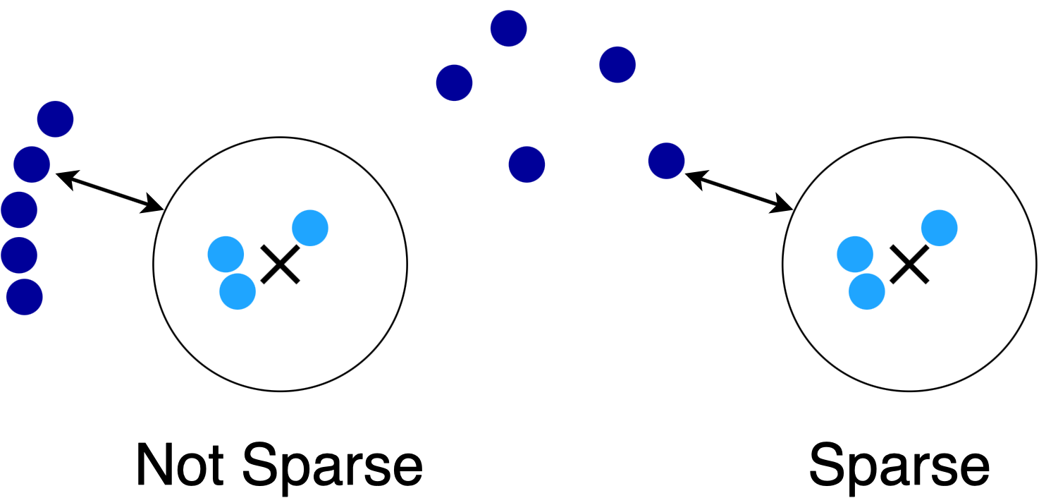
For example, both of these queries are stable, but the query on the right is more sparse than the one on the left because there are fewer nearby points. It turns out that sparse queries are much easier for many algorithms.

Doubling Dimension: There are several measures of “intrinsic dimensionality” for generic metric spaces. Doubling dimension is probably the most well-established condition. The doubling dimension the logarithm of the largest number of balls (of size \(R\)) needed to cover the points in a ball of size \(2R\).

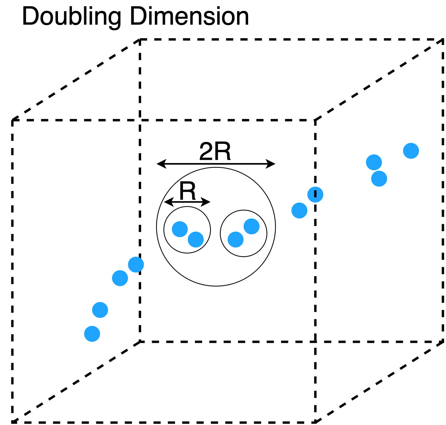
A set of points in \(\mathbb{R}^{d}\) can have a doubling dimension much smaller than \(d\) if large parts of the space are empty. For example, consider the dataset in the picture. All points contained in balls of size \(2R\) can be covered by two balls of size \(R\), so the doubling dimension is \(\log_2(2) = 1\). This agrees with our intuition, since the points lie roughly on a line embedded in 3D space.

In Practice

In practice, near neighbor search implementations are evaluated using information retrieval metrics such as precision and recall instead of their ability to solve the problem statements we discussed earlier. The algorithms are evaluated this way because many applications demand that the search results contain the top \(K\) items in a dataset.

For example, suppose we return 100 points from the dataset as neighbors in a product recommendation engine. A reasonable expectation is that the 10 best (nearest) products appears somewhere in our 100 search results. Unfortunately, the theoretical problem statements are difficult to relate to our real-world expectations from the system. For this reason, we often evaluate algorithms using a metric called “Recall of X at Y” (RX@Y). RX@Y is the fraction of the closest X neighbors that appear in the first Y search results. The values of X and Y are application-dependent. Search engines often use R10@100, while NLP applications like question-answering use R10@10 or even R1@1.

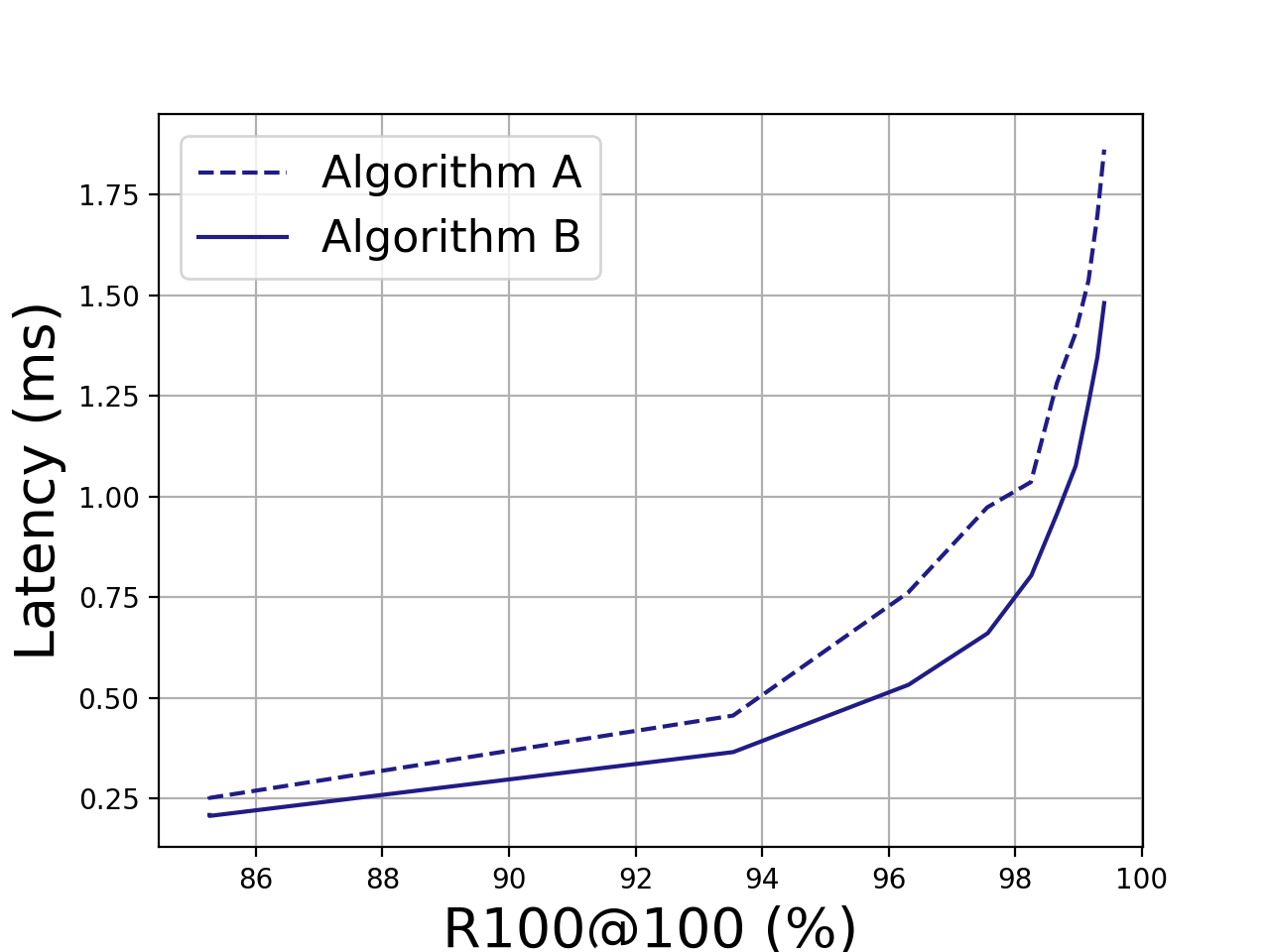
To make it more concrete, consider the performance of Algorithm A and Algorithm B in the figure below.⁵ If our latency budget is 0.75ms, we can get 96% recall with Algorithm A or 98% recall with Algorithm B.

Practical Tradeoffs

If we ask the index to return a fixed number of search results, near neighbor search becomes a tradeoff between recall and query time. The ultimate objective of a search index is to provide the best recall for a given query time budget. Therefore, most people are really solving the JANN problem.

Just-make-it-work Approximate Near Neighbor (JANN): I want an algorithm that finds (enough of) the neighbors without exceeding my latency budget or memory limitations.

In the JANN problem, anything goes - GPUs, deep networks, graph heuristics and parallelism run rampant through modern search algorithms. The truth is that many of the the winning libraries on ann-benchmarks have rock-solid performance without meaningful theoretical guarantees. But it’s still important to discuss the theoretical foundations of the problem, if for no other reason than to understand just what makes the KNN problem so difficult. My hope is that a rigorous analysis of these heuristics will lead to practical improvements as well as deeper insight into the nature of the KNN problem.

Notes

---