People often summarize a “bag of items” by adding together the embeddings for each individual item. For example, graph neural networks summarize a section of the graph by averaging the embeddings of each node [1]. In NLP, one way to create a sentence embedding is to use a (weighted) average of word embeddings [2]. It is also common to use the average as an input to a classifier or for other downstream tasks.
I have heard the argument that the average is a good representation because it includes information from all of the individual components. Each component “pulls” the vector in a new direction, so the overall summary has a unique direction that is based on all of the components. But these arguments bother me because addition is not one-to-one: there are an unlimited number of ways to pick embeddings with the same average. If unrelated collections of embeddings can have similar averages, it seems strange that the mean can preserve enough information for downstream tasks. Yet based on empirical evidence, the overwhelming consensus is that it does.
How can this possibly be a good summary?
Spoiler Warning: The average is a good summary because, under a reasonable statistical model of neural embeddings, there is a very small chance that two unrelated collections will have similar means. The proof involves a Chernoff bound on the angle between two random high-dimensional vectors. We obtain the bound using a recent result on the sub-Gaussianity of the beta distribution [6].
What are embeddings?
An embedding is a map from \(N\) objects to a vector \(x \in \mathbb{R}^{d}\), usually with the restriction to the unit sphere. The objects might be words, sentences, nodes in a graph, products at Amazon, or elements of any other well-defined collection. The key property is that our idea of similarity between objects corresponds to the distance between object embeddings.
For example, suppose you trained a set of word embeddings on the homepage of Florida Atlantic University, where I went to school. The words “Florida” and “Atlantic” nearly always occur together, so these words would have nearby positions in the embedding space.
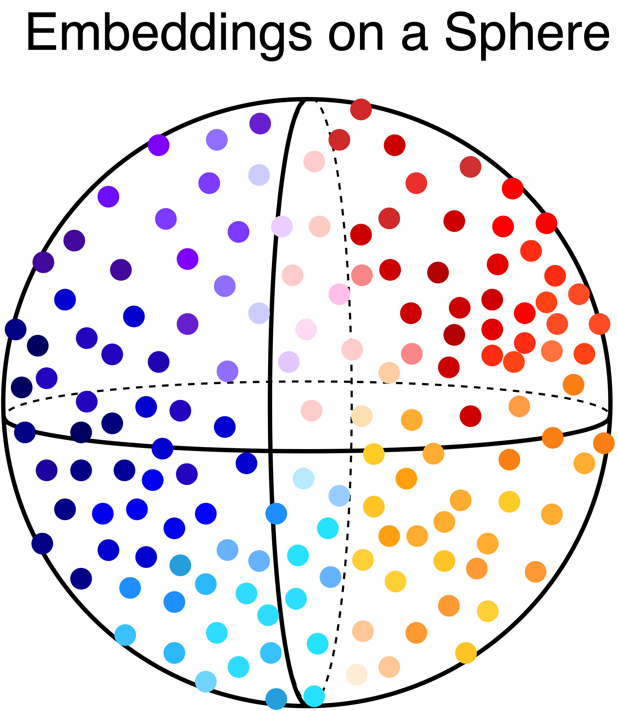
An important empirical observation is that word embeddings tend to be distributed evenly over the surface of the unit sphere when there are enough words in the vocabulary [2]. The intuition behind this phenomenon is that the training process pulls words together when they are similar and pushes dissimilar words apart. After enough “push-pull” cycles, we are left with a fairly uniform set of locations on the sphere. This observation should also hold for other types of embeddings, since most embedding models have similar training objectives.
Collections of Similar Embeddings
Assume we are given a collection of \(m\) object embeddings. We are interested in the relationship between the individual embeddings that compose the collection and the embedding average. For the average to be a good summary, we require the following condition.
Two collections should have similar averages if and only if they share many similar embeddings.
If we have two \(m\)-element collections \(C_1\) and \(C_2\), we can formalize this idea by assuming that each embedding in the first collection can be matched to a nearby embedding in the second collection. The matching process can be understood as pairing every embedding in \(C_1\) with its nearest neighbor in \(C_2\). To simplify the notation, we assume that the collections are sorted so that the first embedding in \(C_1\) matches the first embedding in \(C_2\), and so on.
Definition 1: \(\Delta\)-Similar Collections
We say that two collections of embeddings \(C_1 = \{x_1,x_2,...x_m\}\) and \(C_2 = \{y_1,y_2,...y_m\}\) are \(\Delta\)-similar if the average distance between embeddings is smaller than \(\Delta\).
A straightforward application of the triangle inequality shows that the embedding averages of two \(\Delta\)-similar collections are within distance \(\Delta\) of each other. This shows that two collections with similar embeddings will have similar averages.
Collections of Dissimilar Embeddings
Two collections with unrelated content (i.e. individually dissimilar embeddings) can have exactly the same average embedding because there are \(m\) degrees of freedom in each dimension. The situation is even worse if we consider arrangements that yield similar averages. This breaks the “only if” part of our condition.
However, experiments suggest that this does not happen often - if this behavior were common, then average embeddings would be a poor input feature for graph neural networks and classifiers.
Therefore, our question is: “With what probability do two unrelated collections have mean embeddings with distance \(\leq \Delta\)?”
Spherical Model for Embeddings
Since embeddings are spread evenly over the surface of the unit sphere, we can model embeddings with a uniform spherical distribution. This distribution selects a random point on the surface of the sphere \(S^{d-1}\):
\[S^{d-1} = \{x \in \mathbb{R}^{d}: ||x|| = 1\}\]The uniform spherical distribution is zero-mean and the covariance matrix is \(\frac{1}{d} \mathbf{I}\). The proof comes from the fact that one can generate a random point on \(S^{d-1}\) using
\[x = \frac{z}{||z||} \qquad z \sim \mathcal{N}(0,\mathbf{I})\]See [3] for details.
Central Limit Theorem in High Dimensions
For the purposes of this discussion, we will assume that a collection is formed by drawing \(m\) embeddings i.i.d. from the spherical uniform distribution.
Therefore, we are interested in the average of \(m\) independent samples from \(S^{d-1}\). Since we have i.i.d. random variables, this is a perfect use case for the high-dimensional central limit theorem [4]:
High-dimensional Central Limit Theorem
Let \(X_1, X_2, ... X_m\) be i.i.d. random variables with mean \(\mu\) and covariance \(\mathbf{C}\). Then the sum \(S_m = \sum_{i=1}^{m} X_i\) converges so that:
Applied to this problem, where \(\mu = 0\), we have that the mean embedding converges to a Gaussian distribution. The convergence rate depends on the size \(m\) of the collection.
\[\bar{x} = \sum_{i = 1}^{m} x_i\] \[\bar{x} \to \mathcal{N}\left(0, \frac{1}{dm} \mathbf{I}\right)\]Note that this would have worked even if the embeddings were drawn independently from a symmetric non-uniform spherical distribution. We would still have a zero-mean Gaussian vector for \(\bar{x}\), but we might not have a closed-form expression for the covariance matrix.
Distance between Independent Collections
Using the central limit theorem, we have reduced the problem of finding the distance between mean embeddings to the problem of finding the distance between independent Gaussian random vectors. We will use the angular distance:
\[d(\mathbf{x},\mathbf{y}) = \frac{1}{\pi} \cos^{-1}\left(\frac{\langle\mathbf{x},\mathbf{y}\rangle}{||\mathbf{x}||||\mathbf{y}||}\right)\]Given \(X,Y \sim \mathcal{N}(0,\frac{1}{dm} \mathbf{I})\), we want a probabilistic bound for \(Z\).
\[Z = \frac{\langle\mathbf{X},\mathbf{Y}\rangle}{||\mathbf{Y}||||\mathbf{Y}||} = \left\langle \frac{\mathbf{X}}{||\mathbf{X}||},\frac{\mathbf{Y}}{||\mathbf{Y}||}\right\rangle\]Note that \(Z\) is the inner product between two vectors from the uniform spherical distribution, so the quantity \(X = \frac{Z+1}{2}\) follows a \(\mathrm{Beta}(\frac{d-1}{2},\frac{d-1}{2})\) distribution [5]. Since the Beta distribution is sub-Gaussian [6], we can obtain the following bound for all inner products \(z \geq \frac{1}{2}\). The proof is at the end of the post.
\[\mathrm{Pr}[Z \geq z] \leq e^{-\frac{1}{2}dz^2}\]We can use this result to bound the angular distance between the embedding means:
\[\mathrm{Pr}[\cos^{-1}(Z) \leq \pi \Delta] = \mathrm{Pr}[ Z \geq \cos(\pi\Delta)] \leq e^{-\frac{1}{2} d \cos^2(\pi \Delta)}\]Putting Things Together
We can combine the results for similar and independent collections into a single, concise statement.
Mean Embedding Theorem
Assume we have two collections \(C_1\) and \(C_2\) of \(m\) embeddings on the unit sphere and that \(m\) is large enough to satisfy the central limit theorem. Let \(\bar{x}\) be the average embedding for \(C_1\) and \(\bar{y}\) be the average for \(C_2\). Then
- \(d(\bar{x},\bar{y}) \leq \Delta\) if \(C_1\) and \(C_2\) are \(\Delta\)-similar
- \(d(\bar{x},\bar{y}) \leq \Delta\) with probability \(e^{-\frac{1}{2}d\cos^2(\pi\Delta)}\) if \(C_1\) and \(C_2\) are independent
As a numerical example, consider \(\Delta = 0.4\) and \(d = 128\). Our theorem says that two random collections will have an angular distance smaller than \(0.4\pi \approx 70^{\circ}\) only 0.2% of the time. The plot shows the Chernoff bound for other arrangements of \(d\) and \(\Delta\).
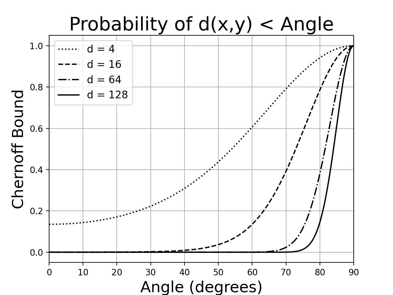
These results make sense because random vectors in high dimensions are nearly always orthogonal. We can see that the angular distance between independent collections strongly concentrates around \(90^{\circ}\), since the probability of a smaller distance drops exponentially with \(d\).
Why is the average a good summary?
The mean is a reasonable way to summarize embeddings thanks to the blessing of dimensionality. Because an exponential number of embeddings are nearly orthogonal in high dimensions, it is unlikely for two independent collections to have similar averages. On the other hand, two related documents are guaranteed to have similar averages. As a result, two collections have similar averages if and only if they share many similar embeddings with very high probability.
Extensions: The results in this post could be extended by analyzing non-uniform and dependent processes to generate the collections. We assumed that that each collection is formed by randomly and independently selecting embeddings from the unit sphere. However, for word embeddings, there is evidence that the selection depends on a latent discourse vector, which represents the topic of the text [2]. In this case, the discourse vectors are selected i.i.d. from the unit sphere, but the embeddings in the document are not. This would require a different application of the central limit theorem.
We could also analyze weighted averages. For example, words are not chosen uniformly but rather but rather according to the term frequency. It would be interesting to explain why the baseline in [2] outperforms the simple average using our probabilistic method.
Proof of the Chernoff Bound
Let \(X = \frac{1}{2}(Z + 1)\) and recall that \(X\) is distributed \(\mathrm{Beta}\left(\frac{d-1}{2},\frac{d-1}{2}\right)\). From [6], we have
\[\mathbb{E}\left[e^{s(X - \frac{1}{2})}\right] \leq e^{\frac{s^2}{16\alpha + 8}}\]Therefore, we can use the (generic) Chernoff bound:
\[\mathrm{Pr}[ X \geq \epsilon ] \leq e^{-s \epsilon}\mathbb{E}[e^{sX}]\]Using the fact that
\[\mathbb{E}[e^{sX}] \leq e^{\frac{s^2}{16\alpha + 8} + \frac{s}{2}}\]For \(1/2 \leq \epsilon \leq 1\), we have
\[\mathrm{Pr}[X \geq \epsilon] \leq e^{\frac{s^2}{16\alpha + 8}- s(\epsilon - \frac{1}{2})}\]Minimizing with respect to \(s\) yields \(s = (\epsilon - \frac{1}{2})(8\alpha + 4)\) and
\[\mathrm{Pr}[X \geq \epsilon] \leq e^{-\frac{1}{2}(\epsilon - \frac{1}{2})^2(8\alpha+4)}\]Now we substitute \(\alpha = (d-1)/2\) and put the inequality in terms of \(Z\):
\[\mathrm{Pr}[\frac{Z+1}{2} \geq \epsilon] \leq e^{-\frac{4d}{2}(\epsilon - \frac{1}{2})^2}\]Put \(z = \frac{\epsilon + 1}{2}\) to get the bound.
References
[1] “Representation Learning on Networks”, Tutorial at TheWebConf 2018, Jure Leskovec, William L. Hamilton, Rex Ying, Rok Sosic. The slides are available here.
[2] “A Simple but Tough-to-Beat Baseline for Sentence Embeddings”, ICLR 2017, Sanjeev Arora, Yingyu Liang, and Tengyu Ma. 2017. [link].
[3] See this answer on CrossValidated for details.
[4] Theorem 3.9.6 in Probability: Theory and Examples (Fourth Edition), Rick Durrett.
[5] See this answer on CrossValidated for details.
[6] “On the sub-gaussianity of the beta and dirichlet distributions” Electronic Communications in Probability, Olivier Marchal and Julyan Arbel. 2017. [link]
[7] “How Well Sentence Embeddings Capture Meaning” ADCS 2015, Lyndon White, Roberto Togneri, Wei Liu, Mohammed Bennamoun. 2015. [link]