Releasing Counts with Differential Privacy

Suppose you want to release count-valued information while preserving the privacy of the people involved in your database. What is the best way to release a differentially private counter? I ask this question because I’ve read several papers that (correctly) claim that the Geometric mechanism is lower-variance than the Laplace mechanism, but it’s not clear whether the difference is large enough to have practical consequences.

Introduction

To motivate the problem, pretend that you’re in a class and the teacher wants to report the number of students who passed the final exam. This seems harmless, but your classroom is full of horrible people. People like Dave. Dave is a jerk who would like nothing more than to identify and harass students who failed the exam.

Dave’s nefarious plan is to ask all of his friends whether they passed the test. If Dave asks enough people, then he can use a process of elimination to figure out whether you failed. He can do this by comparing the number of successful test-takers (which doesn’t include you) with the reported number of students who passed (which does include you). This is called a differencing attack because Dave can determine your exam status by subtracting the two numbers.

Differential privacy

What if we report an approximate count instead of the true one? If we add noise to the count value, the differencing attack is inconclusive: even if you failed, the noise might make it look like you passed (and vice versa). Once noise is added, Dave can’t say for sure whether you failed - even if he knows the exam status of every other student in the class. The best he can do is to calculate the conditional probability that you failed and make an educated guess.

Differential privacy extends this idea for a much broader range of circumstances. If you want a good introduction to differential privacy, Damien Desfontaines has a well-written and informative series of posts over on his blog. The formal definition says that if we have two neighboring datasets \(D\) and \(D'\) that differ in at most one entry, then an \(\epsilon\)-differentially private function \(f(D)\) has the following property:

where the probability is over the randomness in the function \(f(D)\) and \(S\) is any subset of the image of \(f(D)\). In most cases, the \(\in S\) part of the statement simply means that the property has to hold for all of the possible outputs of \(f(D)\). This is certainly true for applications in machine learning, where we usually care about scalar-valued functions over a dataset in \(\mathbb{R}^{d}\).

The parameter \(\epsilon\) is called the privacy budget, and it acts as a limit to the amount of information that \(f(D)\) can leak about any individual element of the dataset. If you read more about differential privacy, you’ll probably also encounter \((\epsilon,\delta)\)-differential privacy. This is a relaxed version of differential privacy where the algorithm might violate the \(\epsilon\) privacy budget for some inputs, but only with probability up to \(\delta\). To get the relaxation, we add \(\delta\) to the right hand side of the privacy property.

Sensitivity

The sensitivity \(\Delta\) of a function is the largest change in \(f(D)\) that we can create by adding or removing a single element from the dataset \(D\). In other words,

Sensitivity is important because it is easy to create a private algorithm once you know \(\Delta\). Among all the ways to achieve differential privacy, the sensitivity method is the most straightforward: there are only two steps! The first step is to find a good upper bound for the sensitivity. The second step is to add noise to \(f(D)\) to create a private output value, a process called output perturbation. The noise depends on \(f(D)\) only through the sensitivity \(\Delta\), and there are standard methods to generate the right amount of noise for any privacy budget \(\epsilon\). As a result, the main challenge is usually to formulate the problem so that the sensitivity is small.

Counting functions are particularly good for the sensitivity method. Each person can only create a change of \(\pm 1\) in the count value, so the sensitivity \(\Delta = 1\). Histograms and frequency counts are therefore good candidates for differential privacy.

The Laplace Mechanism

Additive privacy mechanisms describe ways to generate the noise that we’ll later add to the output of \(f(D)\) to get \(\epsilon\)-differential privacy. The Laplace mechanism is the most common example. To use the Laplace mechanism, we draw noise from the Laplace distribution:

And then we add this noise to the function:

We can usually generate Laplace distributed random variables from standard functions, but if those aren’t available then we can subtract two independent exponential random variables. There’s one problem though: we’re interested in functions that are supposed to output counts. The Laplace distribution outputs real numbers, so we won’t necessarily get a count value if we use it. Fortunately, we can easily fix the problem by rounding the private results toward the nearest integer. This is okay because differential privacy is robust to post-processing.

Variance

The variance of the Laplace mechanism is

For deterministic functions, such as calculating the number of students who passed a test, the error of the private count is determined entirely by the variance of the noise distribution. You can use Markov or Chernoff bounds to make statements like “the private count is within a 10% error margin of the true count, 95% of the time.” The smaller the variance, the better the guarantees.

The Geometric Mechanism

The Geometric mechanism [2] draws noise from the double-geometric distribution, which is the discrete version of the Laplace distribution. Since the distribution is supported by the integers rather than the real numbers, the output value is guaranteed to be an integer. The Geometric mechanism only protects count queries, but the specialization improves performance over the more general Laplace mechanism.

We can generate a double-geometric distributed random variable by subtracting two independent geometric random variables with \(p = 1 - e^{-\epsilon / \Delta}\).

import numpy as np
p = 1 - np.exp(-epsilon)
Z = np.random.geometric(p) - np.random.geometric(p)

Variance

I couldn’t find the variance of the double-geometric distribution anywhere online, but it is easy to derive.

We can show this from the definition of the variance of a discrete random variable. First, observe that \(\mathbb{E}[Z] = 0\) by symmetry, since \(Z = \pm z\) with equal probability for all integers \(z\). Then,

First, the \(z = 0\) term is zero, so we remove it from the summation. The two remaining parts of the sum (from \(-\infty\) to -1 and from 1 to \(\infty\)) are equal, so we can multiply by two and get rid of the absolute value signs. Now we have a type of geometric series sum:

The following fact is well-known to those who know it (just kidding, I used Wolfram Alpha):

The terms cancel nicely and we’re left with

The variance of double-geometric noise is smaller than that of the equivalent amount of Laplace noise. There is a proof at the end of this blog post, but we can also just plot the variance on a log-log scale.

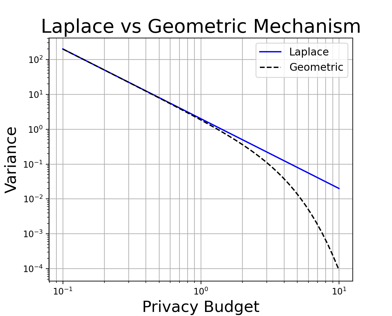
The plot shows that in the low-privacy regime (\(\epsilon \geq 3\)), the variance is over 10x smaller. But for \(\epsilon \leq 1\), the difference is barely noticeable at all.

Experiments

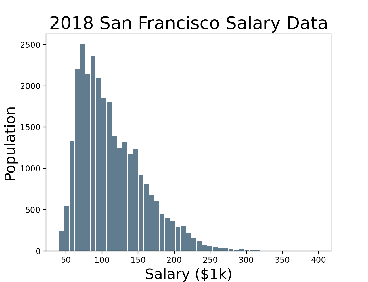
To see whether this really makes a difference, let’s make a differentially private histogram using both mechanisms. We’ll use the (public) San Francisco city employee salary dataset and generate a histogram with 50 bins, ranging from $40k to $400k. The dataset has the salaries for about 29k city employees. Even though it’s not obvious from the histogram, there are a small number of salaries (~10) above $300k.

Next, we perturb each bin with enough noise to preserve \(\epsilon\)-differential privacy. This preserves \(\epsilon\)-differential privacy overall because a single person can only go to one of the bins. In other words, the bins are computed with disjoint sets of data points, so we can apply the parallel composition property.

We do this for many privacy budgets, then plot the \(\ell^{1}\)-error between the noisy private histogram and the ground truth. We average over 500 instances of the noise - the shaded region shows one standard deviation.

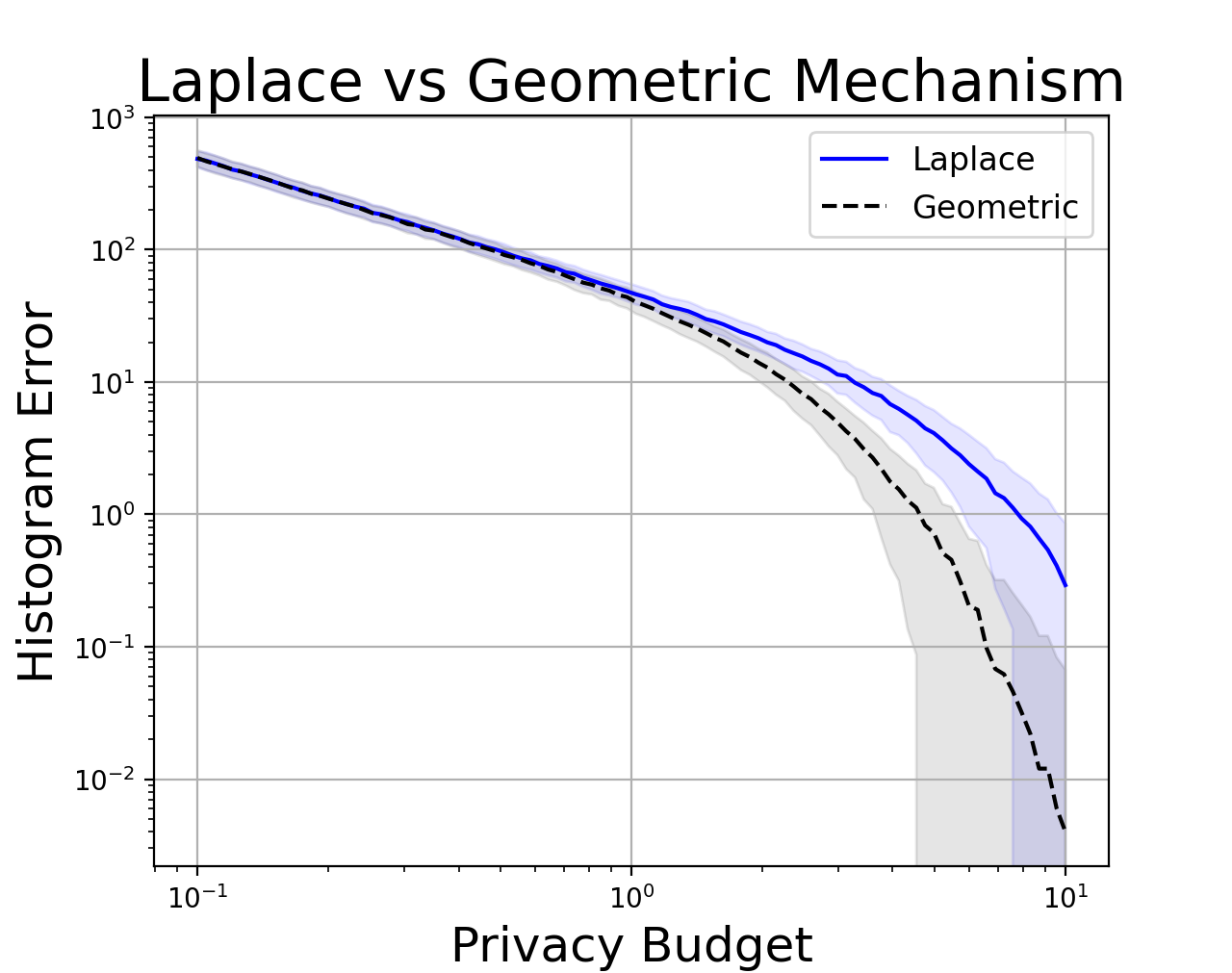
From this plot, I concluded that the practical difference between Laplace and Geometric noise does not substantially affect the results unless you have \(\epsilon > 1\). For better or worse, many industrial systems lie in this region of the privacy-utility tradeoff. Companies usually don’t publish the value of epsilon, which is a contentious issue. However, we do know that Apple uses \(\epsilon = 2\) for health data and \(\epsilon = 4\) for Safari browsing and emoji data (source). Unfortunately, the actual privacy loss might really be much higher - with values up to 14! We also know that Google’s RAPPOR system operates at \(\epsilon \approx 2\). It’s hard to say whether these systems should be made more private, but it’s indisputable that the Geometric mechanism outperforms the Laplace mechanism in this regime.

Of course, the Geometric mechanism is a “free” improvement - and free lunches are few and far between in differential privacy. It’s easy to generate a double-geometric distribution instead of a Laplace distribution, so we should use the mechanism whenever we want to release counts. But the technique isn’t magic and we shouldn’t expect too much unless we’re at a low-privacy operating point of the privacy-utility tradeoff.

Comparison of Geometric Noise and Laplace Noise

We want to show

For convenience, put \(x = \epsilon \Delta^{-1}\) and simplify the inequality to be

Since \(x > 0\), this is equivalent to showing that

Consider the derivative

The derivative is negative everywhere, and the two sides of the inequality are equal when \(x = 0\). This proves the inequality for all \(x \geq 0\).

Notes

[1] I randomly picked this name. If your name is Dave, I’m sorry.

[2] “Universally Utility-Maximizing Privacy Mechanisms” Gosh et al. (STOC’09)

[Photo Credit] Adrien Olichon on Unsplash