In this post, we’ll implement a method to fit a sum of exponential decay functions in Python. The code is at the end of the post. Physical scientists encounter the following problem all of the time. We observe a set of values \(y[n]\) that are generated by multiple exponential decay functions added together and we want to find the individual components of the sum. A climate scientist may do this analyze how different clouds and gasses absorb energy. A chemist may want to identify isotopes in a radioactive sample.
\[y[n] = \sum_{i = 1}^{M} a_i e^{b_i n}\]Unfortunately, fitting exponential sums is hard. It’s so hard that Acton, Princeton computer scientist, gives it an entire section of his well-known essay, “What Not to Compute.” It is best to avoid this problem if possible. For instance, if we know the rates \(b_i\) we can use linear regression instead. If all the \(a_i\) coefficients are the same, we can take the log to get a softmax and use convex optimization. Even if we don’t know \(a_i\) or \(b_i\), it’s a good idea to have as many restrictions as possible to improve our chance of finding a good model. In this post, we’ll deal with the case where \(b_i \leq 0\) (exponential decay) and \(a_i \geq 0\) (positive coefficients).
Prony Method
The Prony method, originally developed in 1795, solves this problem by finding the rates as the roots of a polynomial. Once we have those, we can simply solve for the coefficients via linear regression.
Prony’s method is fast and easy to implement but can misbehave in practice. If we have a sum of decaying exponentials, we do not expect the fitting method to find exponential growth functions or functions that oscillate. Since the rates are found using the roots of a polynomial, \(b_i\) can be positive, negative or complex-valued. Therefore, Prony’s method can produce sums of sinusoids, exponential growth functions, exponential decay functions, and even complex-valued functions! This is undesirable.
While this algorithm will usually find the right coefficients with noiseless measurements, the situation breaks down rapidly when \(y[n]\) is contaminated with noise. Noise completely changes the behavior of Prony’s method. Even a relative error of 1% in \(y[n]\) can be enough to cause serious problems.
Exponential Decay Sum Fit (EDSF)
It turns out that it is hard to find an algorithm that only fits exponential decay functions with positive coefficients. While there is a lot of theoretical work in this area, it is hard to find a concrete algorithm that can do this. I eventually found a method from a 1977 applied physics paper [1], which is a practical appliation of the theoretical results found in [2].
The paper is from 1977, so the computational methods are a little dated. Back then, most computers had less than 16 kB of RAM! The authors put a lot of effort into small optimizations that probably made sense at the time but are unnecessarily complicated today. When I implemented the algorithm, I simplified and eliminated lots of steps.
The algorithm starts by selecting a set of rates \(\theta = e^{b_i}\) and using linear regression to find the corresponding coefficients \(a_i\). Then, we carefully remove the terms with negative coefficients from the model. We repeatedly add and remove terms until the algorithm converges. At convergence, we might have more than M terms, so we merge some of the coefficients to output an M-order model.
Experiment
To compare performance, I generated a 4-term exponential sum with all \(a_i = 1\) and I used 8 samples of \(y[n]\). I added various levels of noise to the samples and fitted \(a_i\) and \(b_i\) with EDSF and Prony’s method. Since Prony often returns complex coefficients, I used the magnitude of the error between the ground-truth parameters and the fit results to measure the error. I used the Python implementation of Prony’s method from here and the EDSF code from this post.
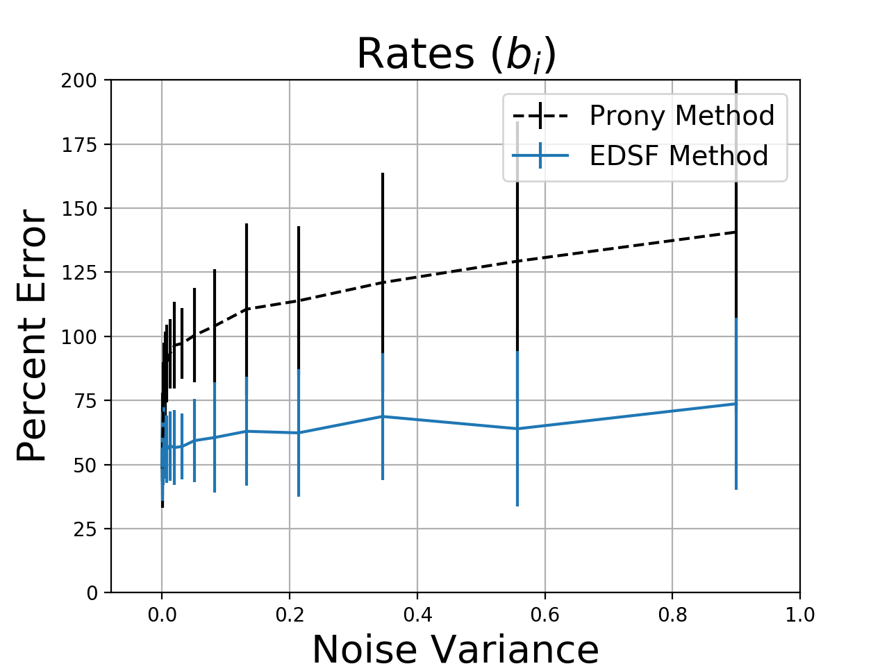
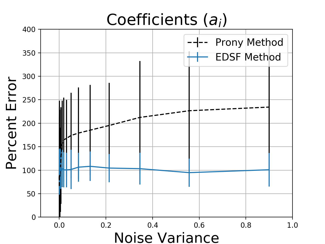
Without noise, Prony’s method is almost exactly correct while EDSF is slightly off. However, as the noise level increases, EDSF more reliably selects parameters that are closer to the true system behavior. Estimation errors of 50% or more are not ideal, but the problem is so sensitive to noise that it is hard to do better. Increasing the number of samples does not help. For both methods, the residual errors were small, but the Prony method produced complex-valued functions and exponential growth about 60% of the time. Since the residual error is small, these techniques might be aceptable for interpolation or modeling even if we cannot reliably recover the true coefficient values.
Python Code
import numpy as np

def E(n,a,theta):
	# Exponential sum function for n and the model (a,theta)
	y = np.zeros_like(n,dtype = np.complex128) # np.float64
	for ai,theta_i in zip(a,theta):
		y += ai*theta_i**n
	return np.abs(y) # return y

def R0(X,n,a,theta):
	# Empirical risk associated with the current model (a,theta)
	return np.sum((X - E(n,a,theta))**2)

def P(grid_thetas,X,n,a,theta):
	# Residual polynomial (from the paper)
	y = np.zeros_like(grid_thetas)
	for ni in n:
		y += 2*(E(ni,a,theta) - X[ni])*grid_thetas**ni
	return y

def linear_stage(A,X):
	# Simple linear regression to find the amplitudes
	sol = np.linalg.lstsq(A, X)
	a_new = sol[0]
	return a_new

def drop_negatives(a_old, a_new):
	# Begin minor iteration to remove negative terms from the fit
	if (np.min(a_new) < 0):
		min_idx = -1 # index k, in the paper
		min_beta = float('inf') # beta_k, in the paper
		for idx, (aoi, ani) in enumerate(zip(a_old, a_new)):
			# aoi = a_old idx, ani = a_new idx
			if ani < 0:
				# guaranteed to be true for one
				# of the amplitudes, see outer "if" statement
				beta = aoi / (aoi - ani)
				if beta < min_beta:
					min_beta = beta
					min_idx = idx
		# Now update a_old
		a_old = (1 - min_beta) * a_old + min_beta*a_new
		a_old[min_idx] = 0
		return (min_idx,a_old)
	else:
		return (None,None)


def coalesceTerms(a, theta, M):
	# Coalesces terms until M terms remain
	N = len(theta)
	if N <= M: # quit if we have M (or fewer) terms
		return (a,theta)
	while N > M:
		# find closest pair
		mind = float('inf')
		minidx = (0,0)
		for i in range(N):
			for j in range(N):
				d = np.abs(theta[i] - theta[j])
				if d < mind:
					mind = d
					minidx = (i,j)

		a_new = a[i] + a[j]
		t_new = 0.5*(theta[i] + theta[j])
		a[i] = a_new
		theta[i] = t_new
		a = np.delete(a,j)
		theta = np.delete(theta,j)
		N = len(theta)
	return (a,theta)


def fitEDSF(y, n, M = None, epsilon_1 = 10e-20, epsilon_2 = 10e-20):
	# fit exponential decay sum function
	# y: the exponential sum fit values to be fitted against
	# n: equally-spaced and contiguous points of n
	#    for instance, n = np.array([1,2,3,4,5,6,7,8])
	# M: model order. If None, then the model runs to convergence.
	#    if given, then the model returns exactly M components
	# epsilon_1: convergence criteria 1 from paper, default works well
	# epsilon_2: convergence criteria 2 from paper, default works well

	# Convergence flags
	converged = False
	R0_old = None
	R0_new = None

	# Parameters
	a_old = np.array([]) # set of amplitude values from previous iter
	a = np.array([]) # set of amplitude values
	theta = [] # theta is a list, need to append often


	iters = 0
	while not converged:
		a_old = a # update previous iteration values

		# 1. Nonlinear part - find a good theta (rate)
		# add theta to minimize the residual polynomial P
		grid_thetas = np.linspace(0,1,100000)
		P_theta = P(grid_thetas,y,n,a,theta)
		idx = np.argmin(P_theta)
		theta_new = grid_thetas[idx]
		theta.append(theta_new)

		# 2. Now set up linear regression problem to find the
		# amplitudes from the system y = A*a
		A = np.zeros((len(n),len(theta)),dtype = np.float64)
		for i,theta_i in enumerate(theta):
			A[:,i] = theta_i**n

		a_new = linear_stage(A,y)
		a_old = np.append(a_old,0)

		# 3. Eliminate terms with negative a_i
		drop_index, a_old = drop_negatives(a_old, a_new)
		while drop_index is not None:
			# delete the negative term
			a_old = np.delete(a_old,drop_index)
			A = np.delete(A,drop_index,axis = 1)
			del theta[drop_index]
			a_new = linear_stage(A,y) # find new a_i
			# ensure new a_i > 0
			drop_index, a_old = drop_negatives(a_old, a_new)


		# 4. Have we converged?
		a = a_new
		R0_new = R0(y,n,a,theta)

		if R0_old is not None:
			E1 = (R0_old - R0_new)/(R0_old)
			if E1 < epsilon_1:
				converged = True

		E2 = P_theta[idx]
		if E2 >= epsilon_2:
			converged = True

		# If we don't have M components
		# keep iterating
		if M is not None:
			if len(theta) < M:
				converged = False
		iters += 1
		if iters > 200:
			converged = True

		R0_old = R0_new

	# Found a good fit, return coefficients
	theta = np.array(theta)
	a = np.array(a)
	if M is not None:
		a,theta = coalesceTerms(a, theta, M)

	final_err = R0(y,n,a,theta)
	return (a,theta,final_err)
You can use this function in two ways. If you provide M, the model will keep merging terms until it has only M exponentials left. This is what we used for the experiments. While this method might not produce the best fit, it will result in a low-order model. If you do not provide M, the model will automatically select the correct order. This results in a lower residual error, but may include a few additional terms. We suggest automatic selection because it usually gets the order correct and has a much lower residual error.
rates = (0.1,0.5,0.8)
N = 10 # number of points
n = np.arange(0,N,1)

y = np.zeros_like(n,dtype = np.float64)
for r in rates[1:]:
	y += r**n

a,theta,err = fitEDSF(y,n) # autoselect M
a,theta,err = fitEDSF(y,n,3) # fit 3-term model
References
[1] Wiscombe, W. J., and J. W. Evans. “Exponential-sum fitting of radiative transmission functions.” Journal of Computational Physics 24.4 (1977): 416-444.
[2] Cantor, David G., and John W. Evans. “On approximation by positive sums of powers.” SIAM Journal on Applied Mathematics 18.2 (1970): 380-388.
[Photo Credit] Adrien Olichon on Unsplash