Recently, I needed a fast FIR filter to remove clutter from the display image of a radar system. We needed to filter each row of our 2D display without decreasing the frame rate. My direct implementation of the difference equation was fast enough, but it made me wonder if I could speed things up further through parallelization.
One common approach is, of course, FFT-based convolution. Given a vector with N elements, the FFT method is \(O(N log(N))\). The difference equation of an M-order FIR filter is \(O(MN)\), so it is reasonable to choose the FFT method when M is sufficiently large. In particular, when M and N are the same order of magnitude, difference equations scale the same as linear convolution - \(O(N^2)\). Typically \(M << N\), so the difference equation is common in practice. For instance, SciPy’s lfilter uses the direct method for FIR filters.
For our 8-order FIR lowpass filter, the time domain method is appropriate since M is much smaller than N. In this case, the algorithm is trivially parallel. We can break the signal into frames and independently filter each frame, provided that we have an overlap between frames of M samples. We need the overlap to eliminate the FIR impulse response, which lasts for M samples after the start of each frame. Since each frame processor only needs read-access to the signal and write access to disjoint chunks of the output, we can assign each frame to a different thread and process multiple frames in parallel. The frame-based approach is common in real-time audio applications, where streaming data is temporarily stored in buffers.
Single-Thread FIR Filter
Our sequential version is implemented in firFilt. The first loop processes the first M elements of the input. This needs a separate loop because x[-1], x[-2], ... x[-M+1] are undefined and are assumed to be zero. Note that this could be made into an IIR filter with minimal code changes.
void firFilt(const double * x, double * y, const double * b, const int N, const int M) {
	int i, j;
	for (i = 0; i < M; ++i) { // zero pad first M elements
		y[i] = 0;
		for (j = 0; j <= i; ++j)
			y[i] += b[j]*x[i-j];
	}
	for (; i < N; ++i) { // full FIR filter from M to N-1
		y[i] = 0;
		for (j = 0; j < M; ++j) // inner loop
			y[i] += b[j]*x[i-j];
	}
}
Parallel FIR Filter
In C++11, the parallel version requires an additional function that will be called by each thread. We can implement this as firThread, a function that performs FIR filtering on a segment of our input. We simply divide x into four parts and give each firThread its own section. I hardcoded the number of threads as four, since that is the number of cores on my machine. We will refer to this implementation as parametric, since the filter coefficients are given as a function parameter.
void firThread(const double * x, double * y, const double * b, const int N, const int M) {
	int i, j;
	for (i = 0; i < N; ++i) {
		y[i] = 0;
		for (j = 0; j < M; ++j)
			y[i] += b[j]*x[i-j];
	}
}
void firFilt4x(const double * x, double * y, const double * b, const int N, const int M) {
	int len = (N - M)/4; // Each frame is of size "len"
	int i, j;
	for (i = 0; i < M; ++i) { // Zero pad first M elements
		y[i] = 0;
		for (j = 0; j <= i; ++j)
			y[i] += b[j]*x[i-j];
	}
	std::thread t1(firThread, x+M, y+M, b, len, M);
	std::thread t2(firThread, x+len+M, y+len+M, b, len, M);
	std::thread t3(firThread, x+2*len+M, y+2*len+M, b, len, M);
	std::thread t4(firThread, x+3*len+M, y+3*len+M, b, N-(3*len+M), M);
	t1.join(); t2.join(); t3.join(); t4.join();
}
I also included hardcoded FIR filters. Rather than loop through an array of filter coefficients, these functions simply multiply x[i] by coefficient values that are known at compile time. In all other respects, they are identical to firFilt and firFilt4x.
Performance Testing
I compiled these functions with the -O3 flag and ran them through a test suite. I used an 8th order low-pass filter for testing. For each value of N, the filter functions were run 500 times and the average execution time was written to a CSV file. The results were processed in Python with Pandas and Seaborn.
	std::mt19937 engine;
	std::uniform_real_distribution<double> dist(-1.0, 1.0);
	int N = 1000;
	int M = 8;
	double * px = new double[N];
	double * py = new double[N];
	double * b = new double[M];
	for (int j = 0; j < N; ++j)
		px[j] = dist(engine);
	// initialize filter
	auto begin = std::chrono::high_resolution_clock::now();
	// call FIR filter
	auto end = std::chrono::high_resolution_clock::now();
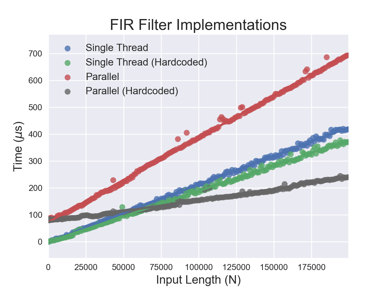
It is understandable for the parallel filters to have a higher y-intercept than the sequential ones. It takes time to set up threads - about 25 μs per thread in this case. It also makes sense that the hardcoded filters are faster, since it’s less likely that we have to load the coefficients from RAM. However, I expected the slope of the line for the single-threaded filter to be four times that of the parallel filter.
This is true for the hardcoded filters, which have a slope ratio of 3.9. However, the parametric filters have extremely surprising behavior! The sequential filter outperforms the parallel one - multithreading causes a performance hit when we don’t hardcode the coefficients. I suspected that memory access and caching might be the culprit, so I conducted some additional tests.
Assembly
Let’s take a look at the assembly for our parallel algorithms. The hardcoded algorithm stores the filter coefficients in the xmm registers and then dereferences x within the loop.
LBB1_4:
	movsd	xmm4, qword ptr [rdx]   # moves x[i] into xmm4
	mulsd	xmm4, xmm0 # 1st coefficient
	movsd	xmm5, qword ptr [rdx - 8] #  moves x[i-1]
	mulsd	xmm5, xmm1 # 2nd coefficient
	subsd	xmm5, xmm4
	# ...
	# And so on, for all the coefficients
	# ...
	movsd	qword ptr [rsi], xmm4 # move sum into y[i]
	add	rdx, 8 # increment the pointer x
	add	rsi, 8 # increment the pointer y
	dec	rax # decrement the loop variable
	jne	LBB1_4
	pop	rbp
	ret # if no jump, then ret
The inner loop of the parametric algorithm loads the filter coefficients each time. It is also worth mentioning that the compiler has done some loop unrolling. The first x[i]*b[i] computation happens before the innermost loop, and each step through LBB0_8 computes two difference equation terms.
LBB0_8: # inner loop
	movsd	xmm2, qword ptr [rbx - 8] # b[i-1] -> xmm2
	mulsd	xmm2, qword ptr [rcx + 8*r14] # rcx = x, r14 = i
	addsd	xmm2, xmm1 # b[i-1]*x[i]
	movsd	qword ptr [rsi + 8*r14], xmm2 # moves into y[i]
	movsd	xmm1, qword ptr [rbx]   # b[i]
	mulsd	xmm1, qword ptr [rcx + 8*r14 - 8] # x[i-1]
	addsd	xmm1, xmm2 # b[i] * x[i-1]
	movsd	qword ptr [rsi + 8*r14], xmm1 # moves into y[i]
	add	rbx, 16 # move rbx by two
	add	rcx, -16 # decrement x by two
	add	rax, -2 # decrement loop variable
	jne	LBB0_8
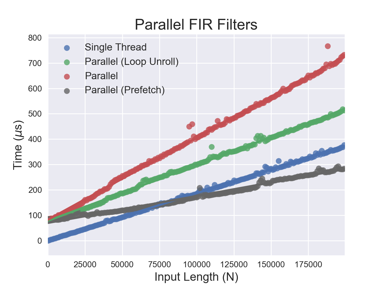
Therefore, there are actually two differences between the fast and slow code - the amount of loop unrolling and the memory access required for the filter coefficients. To examine this behavior further, I tried unrolling four elements of the loop. I also tried prefetching the coefficients into local variables on the stack. It should be noted that the prefetching method requires the filter order at compile time, but not the coefficients.

The results are encouraging and the optimizations definitely reduced the runtime. It is impossible to conclusively say without measuring cache misses, but there is strong evidence that the default parallel implementation generated by the compiler had poor cache utilization. The main algorithmic bottleneck is memory access to the filter coefficients.
Conclusion
Even when an algorithm seems trivial to parallelize, practical implementation details can override theoretical improvements. Here, memory access to a shared resource - the filter coefficients - caused the default parallel implementation to have a higher cache miss rate. Whenever we introduce parallelism to a system, we need to carefully check our assumptions about resource access. Optimizations should always be guided by benchmark and profiler results.